You can’t understand data without controlling the variance.
You can’t control variance without understanding the data.

Variance Doesn’t Go Away By Ignoring It

In an ideal universe, your dataset would contain no bias and only the natural variability you want to analyze. It never happens that way. In fact, most of the “disappointing” statistical analyses you’ll see are more likely to suffer from too much variability rather than too little accuracy. So to get a good result, whether in marksmanship or in data analysis, you have to control variation.

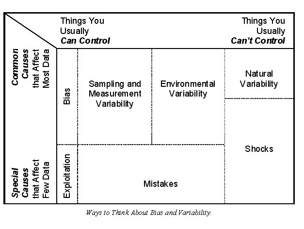
In addition to the sources of variability (see There’s Something About Variance) you can look at variability in terms of how it affects data by:

• Control — the extent to which variability can be controlled so that data aren’t affected.
• Influence — the proportion of data points that are affected by uncontrolled variability.

Sampling and measurement variability usually tend to be under your control. Sometimes you can control environmental variability and sometimes you can’t. These types of variability tend to affect all or most of the data. Natural variability, on the other hand, can’t be controlled and it affects all data. Biases affect all or most of a dataset and usually can be controlled if they are identifiable and unintentional. Intentional bias of only selected data is exploitation. Mistakes and errors may or may not be controllable and they tend to affect only a few data points. Shocks are uncontrollable short-duration conditions or events that can influence a few or even most of the data in a dataset. Examples of shocks include: heavy rainfall upsetting a sewage treatment plant; missing a financial processing deadline so one month has no entry and the next has two; having a meter lose calibration because of electrical interference; mailing surveys without realizing that some have missing pages; assembly line stoppages in an industrial process; and so on.

No one scheme for classifying variance will be best for all applications. Think of variance in terms of the data and the particular analyses you plan to do. You’ll know it’s right because it will help you visualize where the extraneous variability is in your analysis and what you might do to control it.

Three Rs to Remember

The fundamentals of education that we all learned in elementary school are Reading, ‘Riting, and ‘Rithmetic (obviously, not spellin’). With these concepts mastered, we are able to learn more sophisticated subjects like rocket science, brain surgery, and tax return preparation. Similarly, if you plan to conduct a statistical analysis, you’ll need to understand the three fundamental Rs of variance control — Reference, Replication, and Randomization.

Reference

The concept behind using a reference in data generation is that there is some ideal, background, baseline, norm, benchmark, or at least, generally accepted standard that can be compared to all similar data operations or results. References can be applied both before and after data collection. Probably the most basic application of using a reference to control variation attributable to data collection methods is the use of standard operating procedures (SOPs), written descriptions of how data generation processes should be done. Equipment calibration is another well-known way to use a reference before data collection to control extraneous variability.

References are also used after data collection to assess sampling variability. This use of a reference involves comparing generated data with benchmark data. The comparison doesn’t control variability, but allows an assessment of how substantial the extraneous variability is. A more sophisticated use of a reference is to measure highly correlated but differently-measured properties on the same sample, such as total dissolved solids and specific conductance in water. Deviations from the pre-established relationship may be signs of some sampling anomaly. Further, data collected on some aspect of a phenomenon under investigation can be used to control for the variability associated with the measure. Variables used solely to control or adjust for some aspect of extraneous variability are called covariates.

Perhaps the most well known application of a reference is the use of control groups. Control groups are samples of the population being analyzed to which no treatments are applied. For example, in a test of a pharmaceutical, the test and control groups would be identical (on relevant factors such as age, weight, and so on) except that patients in the test group would receive the pharmaceutical and the patients in the control group would receive a placebo.

Replication

If you can’t establish a reference point to help control variability, it may be possible to use replication, repeating some aspect of a study, as a form of internal reference.
Replication is used in a variety of ways to assess or control variability. Replicate sampling or measurements are one example. You might collect two samples of some medium and send both samples to a lab for analysis. Differences in the results would be indicative of measurement variability (assuming the sample of the medium is homogeneous).

In addition to the data source (i.e., sample, observation, or row of the data matrix) being replicated, the type of data information (i.e., attribute, variable, or column of the data matrix) can also be replicated. For example:

• Asking survey questions in different ways to elicit the same or very similar information, such as, Did you like this …, Did this meet your expectations …, and Would you recommend this … .
• Measuring the same property on a sample using different methods, such as pH in the field with a meter and again in the lab by titration.

Replicated samples or variables require a little extra thought during the analysis. If you are looking for a fair representation of the population, a replicated sample would constitute an over-representation. Typically, replicated samples are first compared to identify any anomalies, then, if they are similar, they are averaged. Sometimes, either the first sample or the second sample is selected instead. Never select a sample to use in the analysis on the basis of its value. For replicated variables, first compare the variables to identify any anomalies, then select only one of the variables to use in the analysis. Highly correlated variables will cause problems with many types of statistical analysis (called multicollinearity).

The concept of replication is also applied to entire studies. It is common in many of the sciences to repeat studies, from data collection through analysis, to verify previously determined results.

Randomization

Statisticians use the term “randomization” to refer specifically to the random assignment of treatments in an experimental design, but in its common sense, randomization can involve any action taken to introduce chance into a data generation effort. Randomization is desirable in statistical studies because it minimizes (but not necessarily eliminates) the possibility of having biased samples or measurements. As a consequence, randomization also minimizes extraneous variability that might be attributable to inadvertent inconsistencies in data generation. It is a wonderful irony of nature that introducing irregularities (randomization) into a data generation process can reduce irregularities (variability) in the resulting data.

Out, damn’d variance.

As with replication, randomization can be applied to both samples and variables. Samples or study participants can be chosen at random or following a scheme that capitalizes on their existing randomness. Values for variables that are not inherent to a sample can be assigned randomly. This is done routinely in experimental statistics when study participants are assigned randomly to the treatments. Random assignments are simple to make using random number tables or algorithms.

Variance doesn’t go away by ignoring it. To control variability you have to understand it. But that’s not enough. Data and variance are thoroughly intertwined. You must be proactive in planning your data collection efforts to control as much of the extraneous variability as possible.

Read more about using statistics at the Stats with Cats blog. Join other fans at the Stats with Cats Facebook group and the Stats with Cats Facebook page. Order Stats with Cats: The Domesticated Guide to Statistics, Models, Graphs, and Other Breeds of Data Analysis at Wheatmark, amazon.com, barnesandnoble.com, or other online booksellers.