Ten Fatal Flaws in Data Analysis

Posted on November 7, 2010 by statswithcats

1. Where’s the Beef?

In a way, the worst flaw a data analysis can have is no analysis at all. Instead, you get data lists, sorts and queries, and maybe some simple descriptive statistics but nothing that addresses objectives, answers questions, or tells a story. If that’s all you want, that’s fine. But a data report is not a data analysis. Reports provide information; analyses provide knowledge. It’s like with your bank account. Sometimes you just want a quick report of your balance. That information has to be readily available whenever you might need it and both you and the bank have to be working with exactly the same data. If you want to assess patterns in your spending, though, you have to conduct an analysis. Say you want to figure out how much more you’re spending on commuting over the past five years, you’ll have to compile the data and scrub out anomalies, like the cross-country driving you did on vacation, to look for patterns. Analyses involve much more than a glance (https://statswithcats.wordpress.com/2010/08/22/the-five-pursuits-you-meet-in-statistics/). They take time, sometimes, a lot of time. To make sure you’re getting what you need, look beyond the data tables for models, findings, conclusions, and recommendations. If they’re not there, you didn’t get an analysis.

2. Phantom Populations

If there were to be a fatal flaw in an analysis, it would probably involve how well the samples represent the population. Sometimes data analysts don’t give enough thought to the populations they want to analyze. They use observations to make inferences to a population that doesn’t exist. Populations must be based on some identifiable commonalities that would meaningfully affect some characteristic. A group of anomalies would not be a population. Opinion polls sometimes suffer from phantom populations. Say you surveyed people wearing red shirts. Could you then generalize to everyone who wears red shirts? Canadian researchers found one such phantom population when they tried to create a control group of men who had not been exposed to pornography (http://www.telegraph.co.uk/relationships/6709646/All-men-watch-porn-scientists-find.html). Make sure the population being analyzed is more than an illusion.

3. Wow, Sham Samples

Sometimes the population is real and well defined, but the samples don’t represent it adequately. This is a common criticism of opinion polls, especially election polls. It was the reason cited for why exit polls during the presidential election of 2004 indicated that John Kerry won many precincts that ballot counts later awarded to George Bush. Medical and sociological studies may have sham samples because it is often difficult to select subjects to match some target demographic. Likewise, environmental studies can suffer from inconsistencies between soil types or aquifers. To identify sham samples, look for three things: (1) a clear definition of a real population, (2) a description of how samples were selected so that they represent the population, and (3) information about any changes that occurred during sampling, such as subjects being dropped or samples moved.

4. Enough Is Enough

The number of samples always seems to be an issue in statistical studies (https://statswithcats.wordpress.com/2010/07/17/purrfect-resolution/). For too few samples, question confidence and power; for too many samples, question meaningfulness (https://statswithcats.wordpress.com/2010/07/26/samples-and-potato-chips/). Usually analysts are ready for this question but beware if they cite the old familiar fable about using 30 samples (https://statswithcats.wordpress.com/2010/07/11/30-samples-standard-suggestion-or-superstition/). It may indicate their understanding of statistics is not as formidable as you supposed. Also, if they appear to be using a reasonable number of samples but then break out categories for further analysis, make sure each category has an appropriate number of samples for the analysis they are doing.

5. Indulging Variance

Most people don’t appreciate variance. They don’t even know it’s there (https://statswithcats.wordpress.com/2010/08/01/there%E2%80%99s-something-about-variance/). If their candidate for office is up by two percentage points in a poll, they figure the election is in the bag. Even professionals like scientists, engineers, and doctors don’t want to deal with it. They ignore it whenever they can and just address the average or most common case. Business people talk about variances all the time, only they mean differences rather than statistical dispersion. Baseball players thrive on variance. Where else can you have two failures out of every three chances and still be considered a star? Data analysts have to understand variance and address it at every step of a project. Look for how variance will be controlled in study plans (https://statswithcats.wordpress.com/2010/09/05/the-heart-and-soul-of-variance-control/
https://statswithcats.wordpress.com/2010/09/19/it%E2%80%99s-all-in-the-technique/). Look for variance to be reported with results. And most importantly, look for some assessment of how uncertainty affects any decisions made from the analysis.

6. Madness to the Methods

NASA uses checklists to ensure that every astronaut does things correctly, completely, and consistently. Make sure the analysis you are doing or reviewing takes the same care. If there are multiple data collection points or times, be sure there is a standard protocol or script for generating the data. Be especially concerned if the data are collected over multiple years. Better and cheaper methods and equipment are continuously being developed so be sure they are compatible (https://statswithcats.wordpress.com/2010/09/12/the-measure-of-a-measure/). Be sure the data had been scrubbed adequately of errors, censored and missing data, replicates, and outliers (https://statswithcats.wordpress.com/2010/10/17/the-data-scrub-3/). Finally, be sure the data analysis method is appropriate for the numbers and natures of the variables and samples (https://statswithcats.wordpress.com/2010/08/27/the-right-tool-for-the-job/).

7. Torrents of Tests

If a statistical test is conducted in a study, false positives and false negatives can be controlled, or at least, evaluated. But if there are many tests, you can bet there will be false results just because of Mother Nature’s sense of humor. In groundwater testing, for example, there may be a test for every combination of well, analytes, and sampling rounds, resulting in literally hundreds of tests. There are strategies for dealing with this type of situation, such as hierarchical testing and the use of special tests (look for the term Bonferroni). Be careful of bad decisions based on a small proportion of the tests being (apparently) significant.

8. Significant Insignificance and Insignificant Significance

Here’s where you have to use your gut feel. If a test is statistically significant and you don’t believe it should be, ask about the confidence level and whether the size of the difference is meaningful. Just as correlation doesn’t necessarily imply causation, significance doesn’t
necessarily imply meaningfulness. If something is not statistically significant and you believe it should be, ask about the power of the test and the size of the difference the test should have detected. Be sure the study looked at violations of assumptions (https://statswithcats.wordpress.com/2010/10/03/assuming-the-worst/). Also, look for what’s not there. Sometimes studies do not report nonsignificant results. Such results could be exactly what you’re looking for.

9. Extrapolation Intoxication

Make sure the data spans the parts of the variable scales about which you want to make predictions. If a study collects test data at ambient indoor temperature, beware of predictions made under freezing conditions. Likewise, be careful of tests on rabbits that are extrapolated to humans, maps showing information beyond the limits observed, surveys of one demographic extrapolated to another, and the like. Perhaps the only example of extrapolation that is even grudgingly accepted by statisticians is time-series analysis (https://statswithcats.wordpress.com/2010/08/15/time-is-on-my-side/). You have to extrapolate to predict the future. The issue is how far
into the future is reasonable, which will depend on the degree of autocorrelation, the stability of the data, and the model.

10. Misdirected Models

Models are great tools for helping you understand your data (https://statswithcats.wordpress.com/2010/08/08/the-zen-of-modeling/). Statistical models are based on data. Deterministic models, though, rely on theories, mainly the theories believed by the researcher using the model. But deterministic models are no better than the theories on which they are based. Misdirected models involve researchers creating models based on biased or mistaken theories, and then using the model to explain data or observed phenomena in a way that fits the researchers preconceived notions. This flaw is more common in areas that tend to be more observational than experimental.

Any Questions?

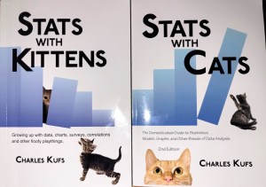
Read more about using statistics at the Stats with Cats blog. Join other fans at the Stats with Cats Facebook group and the Stats with Cats Facebook page. Order Stats with Cats: The Domesticated Guide to Statistics, Models, Graphs, and Other Breeds of Data Analysis at Wheatmark, amazon.com, barnesandnoble.com, or other online booksellers.

Posted in Uncategorized | Tagged cats, extrapolation, information, meaningfulness, measurement scales, model, number of samples, polls, population, precision, resolution, sample size, samples, significance, standardization, statistical analysis, statistical tests, statistics, stats with cats, surveys, uncertainty, variability, variance | 43 Comments

Resurrecting the Unplanned

Posted on October 31, 2010 by statswithcats

Even if you took a class in statistics or another form of data analysis, you probably didn’t hear about frankendata. Frankendata is created when data, collected by different people, at different times and locations, analyzed with different procedures and equipment, and reported in different ways, are conglomerated together to use in a new analysis.

… the cat is cryptic, and close to strange things which men cannot see. –H.P. Lovecraft, The Cats of Ulthar.

In statistics classes, students are provided the same data sets so they all have at least some chance of getting the same answer. Government agencies put great effort into producing consistent data, even while knowing that the data will be harassed, abused, and tortured before the next election. So where does Frankendata come from? Your boss. Your client. Your dissertation adviser. And maybe even your own evil inner twin.

Unlike the saintly sages of statistics who teach in their university utopias, your analysis overlords expect you to be able to make any conglomeration of data into a profitable analysis. Often, this is because your boss sold the client on the idea of cobbling together all the data from the consultants who had the project before your company was hired. The client totally bought into you being able to make sense of the data mishmash.

It is not uncommon that data for a statistical analysis are generated without the prior input of a statistician. Sometimes, even the statistical analysis is an afterthought, coming shortly after the investigator realizes that the data defy interpretation by any means known to him or her. In these cases, you have two possible courses of action. You can try to dodge the bullet, perhaps by explaining the problems with the dataset, and then declining the assignment. This never works. Your Boss wants the Client’s money. The sick-relative gambit works better and is a lot easier to explain, only you can’t use it very often. Most consultants, though, are simply incapable of saying no. This is not just for the money. It’s because they become consultants because they like to solve problems. And believe me, doing a statistical analysis using data that were generated without the oversight of a statistician is a problem.

To non-statisticians, data are data. Concepts like populations and representativeness and randomization and variability aren’t relevant. But data generated without statistical oversight are like cookies made by unsupervised kindergartners. You can’t expect that they followed a recipe since they can’t read yet. You can’t even assume that they know the differences between sugar and salt, or flour and baking powder, or cooking oil and motor oil. You won’t t know what you might have until you take a bite. Scary thought, huh!

So what do you do if faced with this situation? You can swallow hard and not take the assignment. Recognize, though, that someone else will. If it’s an issue that’s important to you, you’ll have more control over what gets done if you’re involved. You might start by following this recipe:

What are the ingredients? — How were samples picked relative to the population of interest? Were any steps taken to minimize variability and bias? How many good samples do you have? Are the variables appropriate for solving the problem? Are outliers and missing data likely to be issues? Can other information be included to augment the analysis?
Is it safe to eat? — What can you do with the data given the number of samples and variables? If a complete analysis isn’t feasible, can an exploratory/pilot study or partial analysis be done?
Where’s the Maalox? — What are the limits/caveats/uncertainties of the analysis? Will the results satisfy the client and other reviewers?

If you can think through an approach that will at least get the client to the next step, it’s probably a good idea to take the assignment. If you do, be sure the client has a clear idea of what you think you can do

I once had a client who was considering buying some property. They were looking at several parcels in an industrialized area of several square miles. The client wanted to know if the groundwater of the area was contaminated because they did not want to get caught up in a regional problem not of their making. The traditional method for answering this type of question would have been to install and sample wells on each property and then develop contour maps for each pollutant of concern. Because of the size of the area and the large number of chemicals to be analyzed for, such an approach would have been prohibitively expensive.

There were, however, scores of industrial facilities in the area that did have groundwater monitoring data, which was publicly available under a State program. The problem was that each site was a different size, from an acre to hundreds of acres, and had different numbers of wells that were sampled on different schedules for different chemical analytes. Each facility used different chemicals, and so, had different monitoring requirements imposed by the State. No analyte was being tested for in even half of the several hundred wells. In a nutshell, nothing was comparable.

Resurrecting this data involved having groundwater specialists review the data from all of the wells in the area. For each of the wells, the specialists determined whether any of the analytes tested for exceeded the standards established by the State. Wells with groundwater that exceeded a standard were coded as 1; wells that did not exceed a standard were coded as 0. The 0s and 1s were then used to produce a contour map of the probability that the groundwater of the area was contaminated. So the client got the information they needed at a price they could afford, and never had to face a village of angry stakeholders with their torches and pitchforks.

Posted in Uncategorized | Tagged cats, frankendata, population, samples, standardization, statistical analysis, statistics, stats with cats | 3 Comments

Tales of the Unprojected

Posted on October 24, 2010 by statswithcats

We have a habit in writing articles published in scientific journals to make the work as finished as possible, to cover up all the tracks, to not worry about the blind alleys or describe how you had the wrong idea first, and so on. So there isn’t any place to publish, in a dignified manner, what you actually did in order to get to do the work.

Richard Feynman, Nobel Lecture, 1966

Communications and relationships always seem to be the biggest problems.

No plan survives implementation. So whether you plan to conduct a data analysis, manage subordinates analyzing data, review results produced by other data analysts, or just have a data analysis conducted for you, there are a few situations that you should be aware of. These are the unexpected events that have little or nothing to do with statistics that can place you in the middle of an awkward if not mean-spirited conflict.

As you might expect, most tales of the unprojected comes down to the quirks of the project participants. Yes, everyone has horror stories of corrupted data, lost files, computer crashes, and the like, but people—how they behave and communicate—are usually what send statisticians screaming in disbelief, frustration, and rage.

Here are seven ways project participants can derail your data analysis project.

The Statistician’s Organization

You would think that communications within your own organization wouldn’t be a big issue. Well, people are people. I once did a project for a manager who said he had an urgent deadline. But first, he delayed a week in providing the data. Then he demanded a partial draft report well ahead of the scheduled review date. He tried to use the hurriedly prepared report to convince his superiors that poor quality work by the staff was making the client dissatisfied. As it turned out, his superiors had already figured out that it was his own incompetence and rude behavior that was upsetting the client. I was lucky; he wasn’t. He was fired shortly after the project was completed successfully. In business, the players don’t wear jerseys. You can’t always tell who’s on your side.

The Client and the Statistician

This is the relationship that you as the statistician have the greatest chance to manage. Usually the relationship is a good one or else you wouldn’t have been selected to do the work. During the project, be sure you are clear on any differences between what the client wants, what the client asks for, and what the client needs. Be sure you are clear on how the client plans to use the results. You don’t want the results misrepresented in a way that will affect your reputation. There are many examples of clients repackaging results in ways you might not expect. I had one client use a report I prepared for a conference presentation. Although he knew nothing about statistics, the karaoke PowerPoint got him management approval to travel on the company’s tab. Fortunately for me, conference attendees tend to zone out when you put numbers on the screen so it wasn’t a big deal. I had another client reuse a spreadsheet I created to conduct some statistical tests on data they supplied. The Client’s Project Manager didn’t realize that I had manually entered some intervening results (viz., tests for Normality and outliers) from another application. That apparently continued for a decade until a new Project Manager from the Client’s office called me to ask how the spreadsheet worked. Sometimes what you don’t know can hurt you.

The Client’s Organization

No matter who your client contact is, he or she works for someone else who in turn works for someone else and so on. Within their organization, then, there may be a variety of competing interests. Even your contact may not be aware of some of the office politics. Management may want a quick answer. Accounting may want documentation of your work before paying you. The legal department may want you to guarantee your results or have your report phrased in certain ways. The plant manager may resent the intrusion of the home office who you work for. I once worked for a client who in turn worked for the ultimate, bill-paying client. The contract I had with my client specified that I had sixteen weeks from the time they supplied the final analysis-ready dataset to complete the analysis. However, my client had agreed to deliver the report to their client by a firm deadline. My client’s project manager held the kickoff meeting and then disappeared leaving the project in the hands of an experienced subordinate. A few months later, the subordinate was reassigned to another project leaving the project to the junior-lever staffer who had been collecting the data. I finally got the data four days, not four months, before the firm deadline specified by my client’s client. Guess who got the blame. So beware, you may be the one who has to accommodate all the different interests in getting your work done.

The Client and the Stakeholders

You and your analysis may never be seen by anyone outside the client’s organization. Your client, on the other hand, may have to make a decision based on your work that is of great interest to shareholders; employees; customers; neighbors; local action groups; the media, and even the public. Consequently, you have to be sensitive to the client’s thinking about how your results will be perceived by the stakeholders. He or she may present your results in simplistic terms that may not be technically correct. I had a client with whom I was conducting an annual employee satisfaction survey. Previous surveys had used five-level scales (i.e., very satisfied, somewhat satisfied, neither satisfied nor dissatisfied, somewhat dissatisfied, and very dissatisfied) which indicated that about forty percent of the employees were satisfied, ten percent were dissatisfied, and about half were sitting on the fence. We wanted to know if the prevalence of neither satisfied nor dissatisfied responses was attributable to apathy or paranoia (there was a no opinion option so that wasn’t a factor), so we switched to a four-level scale by eliminating the middle choice. The responses for the four-level scale indicated that about sixty percent of the employees were satisfied and forty percent were dissatisfied. My client’s boss presented the results to the company’s management and staff as a twenty point improvement in employee satisfaction and nominated several people for company awards. Even the most innocent of actions can invoke the law of unintended consequences.

The Client and the Reviewer

There may be reviewers for your work that are not part of the client’s organization. Some reviewers may be linked to the client, such as a legal firm hired by the client for advice. Other reviewers may be independent or even antagonistic to the client, such as regulatory or law enforcement agencies. Sometimes clients dig in their heels and refuse reviewer requests. This can cause delays that can wreck havoc with your schedule and staffing. Sometimes clients tell you to just give the reviewer whatever he or she wants. This can involve out-of-scope work that might impact your budget. The strangest client-reviewer dynamic I have ever seen involved a client-reviewer relationship that was alternately cooperative and adversarial. When the client was obliging, the reviewer, who represented a regulatory agency, was demanding. When the reviewer was acquiescent, the client was obstinate. I was told to stop work, then start again, then stop, then go. As it turned out, the regulatory agency was trying to extract a larger settlement from the client who, as a large multinational corporation, was perceived to have deep pockets. What the reviewer (and I) didn’t know was that the client was in the process of declaring bankruptcy and was stalling so any settlement with the agency wouldn’t complicate their filing. In the end, there was no settlement, the multinational corporation was liquidated, and the regulatory agency had to start over with the successors. They ended up settling for a small fraction of what the bankrupt client had first offered. You can’t win if everybody is playing by different rules.

The Statistician and the Reviewer

Don’t assume that the reviewer knows as much about statistics as you do. He or she may just have been the only person available to review your work. Even so, most of the time relationships between statisticians and reviewers are fairly straightforward. There may be differences of opinion over an approach or the number or sources of study samples, but usually this relationship is handled professionally by both sides. There are times, though, when inflated egos and hidden agendas cause conflict. One reviewer I worked with agreed to an analysis plan that called for a specific statistical procedure. After the data were collected and the analysis was completed, the reviewer refused to approve the report because “the analysis didn’t work out the way [he thought] it should.” After trying two other procedures with the same result, he relented. On another project that involved a statistical comparison to a control group, the reviewer was surprised that the difference was not significant, even though he had participated in the selection of the control group. He demanded and got a new analysis on new samples from a new control group. The results were the same and he backed down. Yet another reviewer refused to approve an analysis unless published references were provided for the analytical procedure. When the references were provided, the reviewer refused to approve the analysis unless additional statistical studies were done to support the analysis. When the statistical studies supported the analysis, even the reviewer’s support staff encouraged her to approve the analysis. She refused because she “didn’t understand it.” Sometimes, no matter how correct you are, no matter how patient you are, you can’t win.

The Reviewer’s Organization

You usually can’t do much to change interactions in the reviewer’s organization. I’ve had cases in which the reviewer was told to reject the report before it was even submitted. One reviewer I worked with, a university professor contracted with a regulatory agency, provided unusual comments on a statistical analysis. Each part of the review consisted of a few paragraphs of eloquent prose describing some statistical issue related to the analysis followed by one paragraph containing an unintelligible tirade against the analysis, the statistician, and the client. On a hunch, I searched the Internet and found the textbook the professor was using to teach one of his graduate courses. The well-written comments provided by the reviewer were taken verbatim from the textbook. When I informed the Agency the reviewer worked for about his plagiarism, they withdrew the comments but elected not to take any action against the professor. If you can walk away from an engagement with your sanity and a few dollars in your pocket, consider it a success.

Posted in Uncategorized | Tagged bias, cats, client, communications, objectives, politics, polls, project management, relationships, reviewer, statistical analysis, statistics, stats with cats, surveys | 4 Comments

The Data Scrub

Posted on October 17, 2010 by statswithcats

Garbage in, garbage out is a saying that dates back to the early days of computers but is still true today, perhaps even more so. If the numbers you use in a statistical analysis are incorrect (garbage), so too will be the results. That’s why so much effort has to go into getting the numbers right. The process of checking data values can be divided into two parts — verification and validation.

Verification addresses the issue of whether each value in the dataset is identical to the value that was originally generated. Twenty years ago, verification amounted to a check of the data entry process. Did the keypunch operator enter all the data as it appeared on the hard copy from the person who generated the data? Today, it includes making sure automated devices and instruments generate data as they were designed to. Sometimes, for example, electrical interference can cause instrumentation to record or output erroneous values. Verification is a simple concept embodied in simple yet time-consuming processes.

I’m the oversight contractor. Give me all your QA/QC records … and a can of tuna.

Validation addresses the issue of whether the data were generated in accordance with quality assurance specifications. In other words, validation is a process to determine if the data are of a known level of quality that is appropriate for the analyses to be conducted and the decisions that will be made as a result. An example of a validation process is the assignment of data quality flags to each analyte concentration reported by an analytical chemistry laboratory. Validation is a complex concept embodied in a complex time-consuming process.

Changes in data points create a dilemma for statisticians. Change one data point and you’ve changed the entire analysis. It probably won’t change your conclusions, but all those means and variances, and other statistics not to mention the graphs and maps will be incorrect, or at least inconsistent with the final database. This is the most important warning I issue to my clients when I start a job. Still, on the majority of projects, some data point changes after I am well into the data analysis. It’s inevitable.

Finding Data Problems

Lots of bad things can happen in a dataset, so it’s useful to have a few tricks, tips, and tools for finding those mistakes and anomalies.

Spreadsheet Tricks

This is the point when using a spreadsheet to assemble your dataset really pays off. Most spreadsheet programs have a variety of capabilities that are well suited to data scrubbing.

Is that a 0 or an O?

Here are a few tricks:

Marker Rows — Before you do any scrubbing, create marker rows throughout the dataset. You can do this by coloring the cell fill for the entire row with a unique color. You don’t need a lot; just spread them through the dataset. If you make any mistakes in sorting that corrupt the rows, you’ll be able to tell. You could do the same thing with columns but columns usually aren’t sorted.
Original Order — Insert a column with the original order of the rows. This will allow you to get back to the original order the data was in if you need to.
Sorting — One at a time, sort your dataset by each of your variables. Check the top and the bottom of the column for entries with leading blanks and nonnumeric text. Then check within each column for misspellings, ID variants, analyte aliases, non-numbers, bad classifications, and incorrect dates.
Reformatting — Change fonts to detect character errors, such as O and 0. Change the format on any date, time, currency, or percentages and incorrect entries may pop out. For example, a percentage entered as 50% instead of 0.50 would be a text field that could not be processed by a statistical package. This trick works especially well with incorrect dates. Conditional formatting can also be used to find data that fall outside a range of acceptable values. For example, identify percentages greater than 1 by conditionally formatting them with a red font.
Formulas — Write formulas to check proportions, sums, differences and any other relationships between variables in your dataset. Use cell information functions (e.g., Value and Isnumber in Excel) to verify that all your values are numbers and not alphanumerics. Also, check to see if two columns are identical, in which case, one can be deleted. This problem occurs often with data sets that have been merged.

Descriptive Statistics

Even before getting involved in the data analysis, you can use descriptive statistics to find errors. Here are a few things to look for.

Counts — Make sure you have the same number of samples for all the variables. Otherwise, you have missing or censored data to contend with. Count the number of data values that are censored for each variable. If all the values are censored for a variable, the variable can be removed from the dataset. Also count the number of samples in all levels of grouping variables to see if you have any misclassifications.
Sums — If some measurements are supposed to sum to a constant, like 100%, you can usually find errors pretty easily. Fixing them can be another matter. If it looks like just an addition error, fix the entries by multiplying them by

{what the sum should be} divided by {what the incorrect sum is}

For example, if the sum should be 100% and the entries add up to 90%, multiply all the entries by 1.0/0.9 (1.11) and then they’ll all add up to 100%. There will be situations though, especially in opinion surveys, when you’ll have to try to divine the intent of the respondent. If someone entered 1%, 30%, 49%, did he mean 1%, 50%, 49%, or 1%, 30%, 69%, or even 21%, 30%, 49%? It’s like being in Florida during November of 2000. You want to use as much of the data as possible but you just have to be sure it’s the right data.

Min/Max — Look at the minimum and maximum for each variable to make sure there are no anomalously high or low values.
Dispersion — Calculate the variance or standard deviation for each variable. If any are zero, you can delete the variable because it will add nothing to your statistical analysis.
Correlations — Look at a correlation matrix for your variables. Look for correlations between independent variables that are near 1. These variables are statistical duplicates in that they convey the same information even if the numbers are different. You won’t need both so delete one.

There are also other calculations that you could do depending on your dataset, for example, recalculating data derived from other variables.

Plotting

Whatever plotting you do at this point is preliminary; you’re not looking to interpret the data, only find anomalies. These plots won’t make it into your final report, so don’t spend a lot of time on them. Here are a few key graphics to look at.

Bivariate plots — Plot the relationships between independent variables having high correlations to be sure they are not statistically redundant. Redundant variables can be eliminated. Check plots of the dependent variable versus the independent variables for outliers.
Time-series plots — If you have any data collected over time at the same sampling point, plot the time-series. Look for incorrect dates and possible outliers in the data series.
Maps — If you collected any spatially dependent samples or measurements, plot the location coordinates on a map. Have field personnel review the map to see if there are any obvious errors. If your surveyor made a mistake, this is where you’ll find it.

The Right Data for the Job

As it turns out, you’ll probably have to rebuild the dataset more than once, especially if your analysis is complex. You’ll add and discard variables more times than you can count (especially if you don’t document it). Plus, different analyses within a single project can require different data structures. Graphics especially are prone to requiring some special format to get the picture the way you want it. That’s just a part of the game of data analysis. It’s like mowing the lawn. You’re only finished temporarily.

When you do update a dataset, it usually involves creating new variables but not samples. Data for the existing samples might change, for example, you might average replicates, fill-in values for missing and censored data, or accommodate outliers, but you normally won’t add data from new samples. This is because the original samples are your best guess at a representation of the population. Change the samples and you change what you think the population is like. That might not sound too bad, but from a practical view, there are consequences. If you change samples you may have to redo a lot of data scrubbing. The new samples may affect outliers, linear relationships, and so on. It’s not just the new data you have to examine, it’s also how all the data, new and old, fit together. You have to revisit all those data scrubbing steps.

Scrubbing takes time but you have to do it.

Data scrubbing isn’t a standardized process. Some data analysts do a painstakingly thorough job, looking at each variable and sample to ensure they are appropriate for the analysis. Others just remove systematic problems with automated queries and filters, preferring to let the original data speak for themselves. That’s why it’s important to document everything you do. You may have to justify your data scrubbing decisions to a client or a reviewer. You may also need the documentation for contract modifications, presentations, and any similar projects you plan to pursue.

And that’s why it takes so long and costs so much to prepare a dataset for a statistical analysis. Be prepared, it will probably consume the majority of your project budget and schedule but you have to do it so that your analysis isn’t just garbage out.

Posted in Uncategorized | Tagged cats, data scrubbing, statistical analysis, statistics, stats with cats, validation, verification | 15 Comments

Perspectives on Objectives

Posted on October 10, 2010 by statswithcats

And I don’t want a pickerel. / I just want to ride on my motorsickerel.

Conducting a statistical analysis can be like traveling to a foreign country that you’ve never been to before. You had better have a map and some idea of what you want to do there or you might end up wasting a lot of time, get totally lost, or worse, get mugged and end up in the gutter. In a data analysis project, as with any kind of project, you need to be sure you’re clear on your objectives. These define where you’re starting and where you want to end up.

Project goals are usually set out by the client but may be based on regulatory requirements or guidance. Goals may involve:

Conducting a Specific Analysis — Some clients want to interpret their own data but lack the expertise or resources to conduct the analysis. All you might be asked to do is run the software. These assignments are common. Search monster.com for “SAS programmer” and you’ll see what I mean. Sometimes limiting the scope in this manner is a way to simplify a large and complex project. Sometimes, it is used as a way to provide security because no one data analyst would see all the results. Sometimes, it is a way to evade having to share credit with a colleague. Sometimes it’s just what your dissertation adviser wants you to do. Make sure you understand what you’re getting into before you commit.
Answering a Specific Question — Some clients only want one specific thing. Is their new product better than the old product or their competitor’s product? They don’t usually care about what you do so long as you answer the question. Sometimes a client will know what needs to be done, like improve a manufacturing process, but not know where or how to look for solutions. These projects are usually fairly straightforward especially if the requirements are spelled out in some government regulation or guidance document. Just be sure that that’s all you really need to do so you don’t leave your client in the lurch if they aren’t as well acquainted with the requirements as you are.
Addressing a General Need — Some clients have a general notion about what they want but can’t distill it into a specific question or requirement. These cases can be a bit more challenging because you not only have to ascertain what a client thinks they want but also what you believe they need. Projects with general goals often involve model building. You have to establish whether they need a single forecast, map or model, or a tool that can be used again in the future. If the client is looking for a tool, be sure you are clear on the limits of the model’s applicability so there are no misunderstandings or misapplications.
Exploring the Unknown — Every once in a while, a client will have nothing specific in mind, but will want to know whatever can be determined from the dataset. Usually, these projects involve examining large datasets that have been compiled, sometimes over long periods, but never analyzed in total. These projects can be two-edged swords. You can really delve into a dataset and try some of the more esoteric techniques without too much fear of backlash from hostile reviewers. On the other hand, there is usually quite a bit of pressure to come up with something no matter how messy the dataset is. There is also the danger of not being clear on budgets and schedules. Is this a job for statistical modeling, data mining, or just descriptive statistics?

Whatever you do, make sure the goals are SMART — specific, measurable, attainable, relevant, timely — and agreed to by all parties directly involved in the project. There are three situations that can muddy the waters of your objective:

Changing goals are common when the client has only a general goal to begin with. As you find meaning in a dataset during your analysis, the goals may shift or crystallize into something specific. That’s fine. It’s the reason for doing the analysis. Just watch the budget if the redefined objective takes you way beyond your original scope of work.
Multiple goals aren’t uncommon, either. Sometimes, a client might clearly instruct you to consider two or more goals. No problem. Beware of clients looking to get two for the price of one, though. A simple sounding objective might be saddled with additional effort not in your budget; a freebie perhaps only mentioned informally (oh, by the way, can you …), that can substantially affect your performance. A typical example might be something like “conduct this analysis for us, and by the way, can you give us the spreadsheet when you’re done.” You might not even have used a spreadsheet if they hadn’t asked. And it’s one thing if the client just wants the spreadsheet for documentation, but quite another if they plan on using it on a different data set. Doing the calculation might be easy but setting up a spreadsheet to handle the different kinds and amounts of data the client might have in the future would be a much larger effort. You also have to consider what professional liability you may have in such an instance.
Proposals are the third special situation to watch for. Some clients will ask for detailed proposals then say they decided not to do the work. In fact, they just needed a plan for doing the work themselves. They get their cake and eat yours too. You can’t obsess about this. If a client is going to do this, your only option is to decline the work which consultants rarely do unless they know something is afoot. At the same time, you don’t have to give detailed procedures and references for every analysis you might plan to conduct.

If the client isn’t entirely clear about their objectives, it may be that they are unable to articulate their goals in your language of quantitative analysis. So start at the very end. Try asking them what decisions they will need to make based on the results of your analysis. They’ll understand and be able to articulate those decision points. Then you can translate the decisions into the statistical hypotheses you’ll need to evaluate, identify the data you’ll need, and select the appropriate statistical methods.

This is where I wanted to end up.

So if you are contemplating doing a statistical analysis, know where you’re going but be prepared for where you might eventually end up.

Posted in Uncategorized | Tagged cats, goals, objectives, proposals, regulations, SAS, statistical analysis, statistics, stats with cats | 5 Comments

Assuming the Worst

Posted on October 3, 2010 by statswithcats

If you’re going to be poking around data looking for patterns and anomalies, you should be aware of the fundamental requirements you need to fulfill, or at least assume you fulfill. Consider this. All models make assumptions, an evil necessity for simplifying complex analyses. If your model deals in probabilities, like statistical models do, you’ll be making at least five assumptions:

Representativeness – The samples or measurements used to develop the model are representative of the population of possible samples or measurements.
Linearity – The model can be expressed in an intrinsically linear, additive form.
Independence – Errors in the model are not correlated.
Normality – Errors in the model are normally distributed.
Homogeneity of Variances – Errors in the model have equal variances for all values of the dependent variables.

Representativeness

The most important assumption common to all statistical models is that the samples used to develop the model are representative of a population of possible samples that are being investigated. Some statistics books don’t discuss this as a basic assumption because it is viewed as more of a requirement than an assumption. But, obtaining representative samples of populations can be a challenge. Unlike the other assumptions, failure to obtain a representative sample from a population under study would necessarily be a fatal flaw for any statistical analysis. You might not know it, though, because there’s no good way to determine if a sample is representative of the underlying population. To do that, you would need to know the characteristics of the population. But if you knew about the population, you wouldn’t need to bother with a sample. So, representativeness has to be addressed indirectly by building randomization and variance control into the sampling program before it is undertaken. If randomization cannot be incorporated into the sampling procedure in some way, the only alternative is to try to evaluate how the sample might not be representative. This is seldom a satisfying exercise. Making statements like “the results are conservative because only the worst cases were sampled” are usually conjectural, qualitative, and unconvincing to anyone who understands statistics.

Linearity

The linearity assumption requires that the statistical model of the dependent variable being analyzed can be expressed by a linear mathematical equations consisting of sums of arithmetic coefficients times the independent variables. The effects of nonlinear relationships are usually substantial. Applying a linear model to a nonlinear pattern of data will result in misleading statistics and a poor fit of the model to the data. Evaluating the linearity assumption is usually straightforward. Start by plotting the dependent variable versus the independent variables, calculate correlations, and go from there.

This assumption is seldom a problem for three reasons. First, in practice, most models of dependent variables can be expressed as linear mathematical equations consisting of arithmetic sums of coefficients times the independent variables. Second, the assumption will still be met when one or more of the independent variables have a nonlinear relationship with the dependent variable if a mathematical transformation can be found to make the relationship linear. The only catch is that the coefficients (termed the parameters of the model) must still be linear. These models are termed intrinsically linear. In contrast, intrinsically nonlinear models have coefficients that are nonlinear. Third, if a transformation cannot be found to correct a nonlinear relationship, you can still resort to using statistical methods for intrinsically nonlinear models. Nonlinear modeling uses different terminology and optimization processes than linear regression and usually requires specialized software.

Independence

The third assumption common to statistical models is that the errors in the model are independent of each other. Some introductory statistics textbooks describe this assumption in term of the measurements on the dependent variable. There are two reasons for this. First, it’s a lot easier for beginning students to understand, especially if they aren’t familiar with the mathematical form of statistical models and the concept of model errors. Second, and more importantly, the two approaches to describing the independence assumption are equivalent. This is because a data value can be expressed as the sum of an inherent “true” value and some random error. If you have controlled all those sources of extraneous variation, the data and the model errors should be identically distributed.

Say you were conducting a study that involved measuring the temperature of human subjects. Without your knowledge, a well-meaning assistant provides beverages in the waiting room – piping hot coffee and iced tea. When you plot a histogram of the temperature data, you might see three peaks (called modes), one centered at 98.6°F, another at a degree or so higher and a third a degree or so lower. Your data have violated the independence assumption. The subjects who drank the coffee all had their temperatures linked to the higher temperature of the coffee. The subjects who drank the iced tea all had their temperatures linked to the lower temperature of the iced tea. What are the chances you might notice this dependency? If you had a dozen or so subjects, the chances wouldn’t be good. With 100 subjects, you might notice something. With 1,000 subjects, you would almost certainly notice the effect, though if you’re providing beverages to 1,000 subjects, you might consider getting out of research and opening a coffee shop.

Assessing independence involves looking for serial correlations, autocorrelations, and spatial correlations. A serial correlation is the correlation between data points with the previously listed data points. For example, making measurements with an instrument that is drifting out of calibration will introduce a serial correlation. Spatial or temporal dependence are often present in environmental data. For example, two soil samples located very close together are more likely to have similar attributes than two samples located very far apart. Likewise, two well water samples collected a day apart are more likely to have similar attributes than two samples collected two years apart.

Most statistical software will allow you to conduct the Durban-Watson test for serial correlation as part of a regression analysis. For temporally related data, correlograms are used to assess autocorrelations and partial autocorrelations. Spatial independence can be evaluated using variograms, plots of the spatial variance versus the distances between samples. Correlograms and variograms require specialized software to produce and some experience to interpret.

When the independence assumption is violated, the calculated probability that a population and a fixed value (or two populations) are different will be underestimated if the correlation is negative, or overestimated if the correlation is positive. The magnitude of the effect is related to the degree of the correlation.

Some people confuse the independence assumption, which refers to model errors or measurements of the dependent variable, with the assumption that the independent variables (AKA, predictor variables) are not correlated. Correlations between predictor variables, termed multicollinearity, are also problematical for many types of statistical models because statistics associated with such models can be misleading.

Normality

The Normality assumption requires that model errors (or the dependent variable) mimic the form of a Normal distribution. This assumption is important because the Normal model is used as the basis for calculating probabilities related to the statistical model. If the model errors don’t at least approximate a Normal distribution, the calculated probabilities will be misleading. It would be like trying to put a square peg into a round hole.

There are many methods for evaluating the Normality of a distribution, which fall into one of three categories:

Descriptive Statistics – Including the coefficient of variation (the standard deviation divided by the mean), the skewness (a measure of distribution symmetry), and the kurtosis (a measure of relative frequencies in the center versus the tails of the distribution). If the coefficient of variation is less than about one, and the skewness and the kurtosis are close to zero, it’s reasonable to assume the errors approximate a Normal distribution
Statistical Graphics – Statistical graphics are more revealing than descriptive statistics because they indicate visually what data deviate from the Normal model. Interpreting these graphics can be somewhat subjective, however. The most commonly used statistical graphics are histograms,box plots,and probability plots. Other statistical graphics sometimes used to evaluate Normality include stem-and-leaf diagrams, dot plots, and Q-Q plots.
Statistical Tests – Statistical tests are more rigorous than either descriptive statistics or statistical graphics. Commonly used tests of normality include the Shapiro-Wilk test, the Chi-squared test, and the Kolmogorov-Smirnov test. One of the problems with statistical tests of Normality is that they become more and more sensitive as the sample size gets large. So, a statistical test may indicate a significant departure from Normality that is so minor it is unimportant. Thus, tests of normality may be definitive but irrelevant.

So how should you evaluate Normality? Focus on one method or decide on the basis of a preponderance of the evidence? First, you have to understand that statistical tests, statistical graphics, and descriptive statistics are like advisors. They all have an opinion, none is always correct, and they sometimes provide conflicting advice.

One approach to evaluating Normality is to first look at a histogram to get a general impression of whether the data distribution is even close to a Normal distribution. If it is, look at a test of Normality, preferably a Shapiro-Wilk test. This test assumes Normality so if there’s no significant difference, you can conclude that the data came from a Normally distributed population. If there is a significant difference, then your decision becomes problematical. Look at a probability plot to determine where the departures from Normality are. You might have a problem if the deviations are in the tails because that’s where the test probabilities are calculated. If there is an appreciable deviation from Normality in the tails of the distribution of errors, consider transforming the dependent variable or using a nonparametric procedure.

Equal Variances

The last assumption, termed homoscedasticity, means that the errors in a statistical model have the same variance for all values of the dependent variable. For models involving grouping variables, the assumption means that all groups have about the same variance. For models involving continuous-scale variables, homoscedasticity means that the variances of the errors don’t change across the entire scale of measurement.

For example, in the case of a measurement instrument, homoscedasticity requires that the error variance be about the same for measurements at the low, middle, and high portions of the instrument’s range, which can be a difficult requirement to meet. Another example would be measurements made over many years. Improvements in measurement technologies could cause more recent measurements to be less variable (i.e., more precise) than historical measurements.

Assessing homoscedasticity is more straightforward for discrete-scale variables than for continuous-scale variables because there are usually more than a few data points at each scale level. A simple qualitative approach is to calculate the variances for each group and look at the ratios of the sample sizes and the variances. There are also more sophisticated ways to evaluate homoscedasticity, such as Levene’s test.

Violations of the homoscedasticity assumption tend to affect statistical models more than do violations of the Normality assumption. Generally, the effects of violating the homogeneity-of-variances assumption will be small if the largest ratio of variances is near one and the sample sizes are about the same for all values of the independent variables. As differences in both the variances and the numbers of samples become large, the effects can be great. Violations of homoscedasticity can often be corrected using transformations. In fact, transformations that correct deviations from Normality will often also correct heteroscedasticity. Non-parametric statistics also have been used to address violations of this assumption.

So, you don’t have to assume the worst might happen in violating a statistical assumption. The effects may be minor or there may be an alternative approach you can use. You just have to know what to look for.

Posted in Uncategorized | Tagged cats, errors, homoskedasticity, measurement, Normal distribution, Normality, population, probability, Representativeness, statistical analysis, statistical assumptions, statistics, stats with cats, variance, violations of assumptions | 17 Comments

It was Professor Plot in the Diagram with a Graph

Posted on September 26, 2010 by statswithcats

I’m looking for clues.

You probably were taught how to graph data in high school. Depending on your work, you may frequently plot data yourself or look at graphs prepared by others. Even if you don’t use graphs on your job, you may run into them during your leisure time, reading the newspaper, managing your finances, or playing Dungeons and Dragons. But there’s a big difference between looking at someone else’s graph and preparing one yourself. When you were learning how to graph in school, the teachers told you what kind of graph to use. They gave you carefully selected data that was matched to the graph you were supposed to create. There was help available if you had any questions. Now, it’s just you and your computer. So if you have no clue as to where to begin, here are a few tips that may help.

First let’s get past the jargon of plots, charts, graphs, and diagrams. All of these terms are defined as visual representations of data. All are used synonymously. All are used as both nouns and verbs. All have other meanings. To split hairs:

Plots tend to place more emphasis on individual data points.
Charts tend to involve lines and areas more than individual points.
Graphs tend to be more mathematically complex than charts and plots.
Diagrams tend to be more artistic and fill the entire data space.

Not everyone would agree with this, of course. That being said, you can usually refer to visual representations of data by any of the four terms without being called out by a smart-aleck critic. If you’re referring to a specific kind of visual representations of data, one of the four terms usually is preferred, for example, bar charts, scatter plots, and block diagrams. Most specific kinds of visual representations of data are called plots or charts, and to a much lesser extent, diagrams. The term graph is used mostly in a general sense, which is how it is used in this blog.

A Graph a Minute

The first thing you’ll need to do is figure out what kinds of graphs you could draw. Start by answering these questions:

Is your focus on variables or samples? Do you want to show how a number of samples are related to each other on the basis of one or more variables or do you want to show how a number of variables are related to each other for a very small number of samples?
Will you plot individual points or group means? How many data points do you have to plot? Do you want to show the points individually or do you want to show the averages of groups of data points (this is useful when you have a large number of data points)?
What is the aim of the graph? There are many reasons to plot data and most graphs have multiple goals. For simplicity, decide whether the primary aim is to show:
- Data frequency and distribution
- Relative proportions of the components of a mixture
- Properties or values of data points
- Trends, patterns, or other relationships among variables.
How many axes will you need? How many variables do you have? Are they measured on the same or different scales? Are the scales discrete or continuous?

Once you can answer those questions, you can use this table to help you choose some of the more common kinds of graphs to try with your data. There are, of course, a virtually uncountable number of kinds of graphs, subspecies of graphs, variations and extensions of graphs, and combinations of graphs. To start, focus on simple graphs you can get from the software you have available. Later, you can prepare the Piper plots you used to justify your purchase of that specialized piece of software you wanted.

Common Types of Graphs for General Data Analysis.

			Data Scales
Chart	Used to Show	Chart Axes	Horizontal Axis	Vertical Axis	Additional Axes	Availability
Box Plot	Distribution	Rectangular	Categorical, continuous (sample size)	Continuous		Specialized software
Dot Plot	Distribution	Rectangular	Ordinal, continuous	Ordinal		Specialized software
Histogram	Distribution	Rectangular	Ordinal, continuous	Ordinal		Spreadsheet software
Probability Plot	Distribution	Rectangular	Ordinal, continuous	Continuous		Specialized software
Q-Q Plot	Distribution	Rectangular	Ordinal	Ordinal		Specialized software
Stem-Leaf Diagram	Distribution	Rectangular	Ordinal	Ordinal, continuous		Specialized software
Ternary Plot	Mixtures	Triangular	Continuous (percentages)	Continuous (percentages)	Continuous (Percentages)	Specialized software
Pie Chart	Mixtures	Circular	Categorical	Continuous (percentages)		Spreadsheet software
Area Chart	Properties	Rectangular	Ordinal, continuous	Continuous		Spreadsheet software
Bar Chart	Properties	Rectangular	Categorical	Continuous		Spreadsheet software
Candlestick Chart	Properties	Rectangular	Continuous	Continuous		Develop from scatter plot
Control Chart	Properties	Rectangular	Continuous	Continuous		Specialized software
Deviation Plot	Properties	Rectangular	Continuous	Continuous		Develop from scatter plot
Line Chart	Properties	Rectangular	Categorical, ordinal	Continuous		Spreadsheet software
Map	Properties	Rectangular	Continuous	Continuous	Any	Specialized software
Matrix Plot	Properties	Rectangular	Nominal	Nominal	Text	Develop from table
Means Plot	Properties	Rectangular	Continuous	Continuous		Develop from scatter plot
Spread Plot	Properties	Rectangular	Continuous	Continuous		Develop from scatter plot
Block Diagram	Properties	Cubic	Nominal	Nominal	Nominal	Specialized software
Rose Diagram	Properties	Circular	Ordinal, continuous	Continuous		Specialized software
Multivariable Plot	Relationships	Rectangular, circular, other	Any	Continuous	Continuous	Specialized software
Bubble Plot	Relationships	Rectangular	Continuous	Continuous	Continuous	Spreadsheet software
Contour Plot	Relationships	Rectangular	Continuous	Continuous	Continuous	Specialized software
Icon Plot	Relationships	Rectangular	Continuous	Continuous	Multivariable plot^*	Specialized software
Scatter Plot: 2D	Relationships	Rectangular	Continuous	Continuous		Spreadsheet software
Scatter Plot: 3D	Relationships	Cubic	Continuous	Continuous	Continuous	Specialized software
Surface Plot	Relationships	Cubic	Continuous	Continuous	Continuous	Specialized software
* (e.g., Radar Plot, Sun Chart, Star Plot, Side-by-side bar charts, Polygon Plot, Sparklines, Chernoff faces)

You Can’t Spell Chart without Art

There are competing philosophies of graphing, divided to some extent by perceptions about the audience for a graph. The philosophy of many art directors of newspapers and magazines is to keep the graph simple, interesting, and attractive in order to engage the reader. Look no further than USA Today, Newsweek, or Time to see three dimensional exploded pie charts and bar charts made of little soldier icons or dollar bills or some other cutesy graphic. In contrast, Edward Tufte, perhaps the preeminent expert in informational graphics, espouses a philosophy that assumes the audience is knowledgeable and interested. Graphs should provide as much information as needed as efficiently as possible. Tufte makes many good points in his books, The Visual Display of Quantitative Information (1983, 2001), Envisioning Information (1990), Visual Explanations (1997), and Beautiful Evidence (2006), including:

The dimension of a chart must not be greater than the dimension of the data. For example, if you’re plotting two variables on a Cartesian (rectangular) graph, don’t add an extra axis (dimension) for depth. It may be visually appealing but it’s scientifically misleading.
Data must be presented in context. You shouldn’t show just part of a data set.
Label everything you need to make sure the data are presented accurately and meaningfully.
Maximize the data density and the data-ink ratio. Put enough data in your graph to make it worthwhile. Eliminate everything on the chart that isn’t data or contributes to the interpretation of the data.
Eliminate chart junk, the unnecessary pictures, dimensionality, grid lines, fill patterns, and other objects that clutter a graph while adding no scientific value.

Tufte believes he has the audience’s attention while the art directors believe they have to compete for it. Then there are authors like David McCandless (www.informationisbeautiful.net) who look at presenting data from an artistic perspective. Their graphics are truly works of art though the graphs are based on data and aimed at engaged audiences. All of these graph developers make valid points. They simply have different perspectives, different audiences, different aims, and different data.

Posted in Uncategorized | Tagged axis, cats, charts, diagrams, graphs, jargon, McCandless, measurement scales, number of samples, plots, statistical analysis, statistics, stats with cats, Tufte | 12 Comments

It’s All in the Technique

Posted on September 19, 2010 by statswithcats

To err is human, to purr feline. Robert Byrne

You can’t understand your data unless you control extraneous variance attributable to the way you select samples, the way you measure variable values, and any influences of the environment in which you are working. Using the concepts of reference, replication and randomization, you can control, minimize, or at least be able to assess the effects of extraneous variability in five ways:

Procedural Controls — used primarily to prevent measurement variability by reference.
Quality Samples and Measurements — used primarily to identify sources of measurement and environmental variability by reference.
Sampling Controls — used primarily to correct sampling variability by reference and randomization.
Experimental Controls — used primarily to correct measurement and environmental variability by reference and randomization.
Statistical Controls — used primarily to correct environmental variability by reference.

Procedural Controls

Procedural controls include the field, office, and laboratory procedures that specify how activities related to data generation should be carried out. Forms of procedural control include Standard Operating Procedures (SOPs), chain-of-custody (CoC) procedures, survey scripts and instructions, checklists, calibration procedures, training courses and so on. Procedural controls are the main way to minimize extraneous variation before it occurs.

Quality Samples and Measurements

When a physical sample is collected, especially for laboratory analysis, there are a variety of samples that can be collected to verify that the analyses produce valid results. The aim of quality tests is to identify quality problems and sources of undesirable variability. Some quality samples and tests allow corrections to data points to correct bias. Quality samples used to assess variability in the collection and measurement of the experimental samples include:

Replicate samples — multiple samples collected of the same subject to assess variability. Replicate samples may be collected by splitting a large sample into two or more subsamples (called split samples). Alternatively, discrete samples may be collected sequentially (called co-located samples). Most replicates are co-located samples because they are less time-consuming to collect. Co-located samples of mixable media (e.g., fluids like water and air) will usually be very similar compared to co-located samples of non-mixable media (e.g., solids like soil). Duplicate is a generic term for a replicate sample that may be either a split sample or a co-located sample.
Blind samples — split samples submitted with unique sample identifiers so they appear to be from different sources. Blind samples are an independent check of laboratory methods.
Trip blanks — distilled water placed in sample containers and sealed in the lab. Trip blanks are carried by the field sampling team and returned to the lab with the test samples. If any aspect of the sample handling and transport process might have compromised the quality of the samples within their containers, the effect should be detectable in the trip blank. It is very rare for trip blanks to contain contaminants.
Rinse blanks — distilled water that has been poured over reusable sampling equipment that has been decontaminated. Rinse blanks are sometimes called field blanks, rinsate blanks, equipment blanks, or decontamination blanks because they are a test of the cleanliness of the sampling equipment.
Atmosphere blanks — distilled water placed in sample containers that are opened during sample collection. Atmosphere blanks are a test of whether any air pollutants or windblown particulates might have contaminated test samples during the process of collecting the samples.
Water blanks — potable water used for site activities, particularly rock drilling. Water blanks are also collected from wells when domestic plumbing is being assessed for lead contamination.
Preservative blanks — preserved samples of distilled water. Preservative blanks are used to assess possible contamination of the acids, bases, and other reagents used to preserve test samples.

Analytical results from these samples are usually checked during data validation and exploratory data analysis. Except for replicates and blind samples (which are usually averaged), they are not included in datasets to be used for statistical analysis. Other QA/QC samples used to check laboratory procedures include:

Laboratory blanks — distilled water or purified solid prepared in the lab to assess contamination from reagents, glassware, and analytical hardware. These samples are sometimes called method blanks because they are a test of the laboratory method.
Performance evaluation samples — samples containing known concentrations of specific compounds. PE samples are usually used to certify laboratories for a particular type of analysis rather than check quality on a specific data collection task.
Calibration samples — samples containing known concentrations of an analyte similar in chemical behavior to the analytes of interest. These samples are used to calibrate instruments and assess method bias.
Matrix spikes — samples of the media being analyzed that have been spiked with known concentrations of a representative analyte. These samples are used to check for interferences between the analytes being tested and the sample matrix. Matrix spike duplicates are routinely analyzed by laboratories to assess measurement variability.

Analytical results from these samples are usually checked during data scrubbing. They are not included in datasets to be used for statistical analysis. Most of these QA/QC samples are used only for chemistry laboratories. Quality samples for other types of laboratory analyses (e.g., geotechnical, radiological, biological) are usually limited to replicates.

These are commonly used quality samples but there are many others possible. You create the samples to fit the experimental situation. Don’t feel limited to laboratory samples. You can use the same approach to create tests or other methods of variance assessment. If you understand the possible sources of variation in your data, you can create relevant quality tests for survey questions, industrial processes, or whatever your study will involve.

Sampling Control

Some types of samples have inherent properties that may introduce extraneous variability into data being generated. For instance, differences in sex, age, and social class, may introduce extraneous variability in sociological surveys. Environmentally related examples might include: soil type, geologic strata, species, location and depth, and season (or other time unit). Applying sampling controls involves grouping the data by the control factor and calculating statistical analyses for each homogeneous group. Stratified sampling designs are one form of sampling control.

Sampling controls can be used to prevent, identify, or correct all kinds of extraneous variation. As a consequence, they are used to some extent in most statistical studies.

Experimental Control

Statistical studies can be categorized into two types — observational and experimental. In an observational study, the phenomenon under investigation is a characteristic of the objects being sampled. The concentrations of arsenic in the soils of a waste management facility would be an example. Variability and bias in observational studies can be assessed through the use of control samples. Control samples (like quality samples) are groups of samples that don’t have the condition being tested but are otherwise identical to the experimental group. Adding an offsite (or background) area to the study of the waste management facility would be an example of a control group.

In an experimental study, the phenomenon under investigation is assigned to the objects being sampled. Testing a pollution cleanup technique on several plots of contaminated soil would be an example of an experimental study. In such a study, the cleanup techniques would be randomly assigned to the plots in a manner that would help control some of the variation in the plots.

So, the difference between experimental and observational studies is that in an:

Experimental study, samples are randomly assigned to controlled conditions.
Observational study, samples are randomly selected from preexisting conditions.

I’m not telling who got the placebo. (Cat stays in bag.)

Another way to control variability and bias is through the use of placebos. A placebo is usually thought of as a faux drug because of its association with statistical tests of pharmaceuticals, but it can be any item or action that gives the appearance of being a valid treatment. For example, give two patients blue pills, one of which has some active ingredient and the other does not. To test a new pesticide, spray two agricultural test plots, one of which contains the pesticide and the other contains just water. The key is that the subject or data generator can’t tell the difference. In Season 5, episode 14 of the television series House, the nurse can tell which patients are being given the placebo during Dr. Foreman’s drug trial because the real pharmaceutical has a strong odor. This would not be a good example of an effective placebo.

Placebos are a type of blinding. In any experiment, there are subjects or samples, experimenters, data collectors or generators, and data analysts. Sometimes, one individual will fill several roles, such as the experimenter who designs the experiment and then generates and analyzes the data. But whenever there are humans involved, there exists the possibility of intentional or unintentional bias. Blinding is simply the act of denying one or more of the study participants with information that might induce them to behave differently.

To test the effects of a pharmaceutical, for example, a single-blind study might involve not telling subjects whether they are receiving the active drug or a placebo. A double-blind study might involve not telling either the subjects or the data generators (the nurses who collect physical measurements on the subjects or the lab technicians who analyze blood samples) who received the drug and who received the placebo. A triple-blind study might involve not telling the subjects, the data generators, or the data analysts who received the drug and who received the placebo. It’s ironic that the less informed the participants are, the better the statistics. Too bad government doesn’t work that way.

Statistical Control

Special statistics and statistical procedures can be used to partition variability shared by measurements so that extraneous variability can be assessed. For example, partial correlations quantify the relationship between two variables while holding the effects of other variables constant. A covariate is a continuous variable that is incorporated into an analysis of variance design to eliminate extraneous variability so that tests of the grouping factors will be more sensitive. Statistical controls are typically used when variation cannot be controlled adequately through other means.

Posted in Uncategorized | Tagged bias, blinding, cats, control sample, covariate, jargon, measurement, placebo, precision, samples, SOP, statistical analysis, statistics, stats with cats, uncertainty, variability, variance, variance control | 11 Comments

The Measure of a Measure

Posted on September 12, 2010 by statswithcats

If you can measure a phenomenon, you can analyze the phenomenon. But if you don’t measure the phenomenon accurately and precisely, you won’t be able to analyze the phenomenon accurately and precisely. So in planning a statistical analysis, once you have specific concepts you want to explore you’ll need to identify ways the concepts could be measured.

All feline phenomena should be measured with appropriate scales.

Start with conventional measures, the ones everyone would recognize and know what you did to determine. Then, consider whether there are any other ways to measure the concept directly. From there, establish whether there are any indirect measures or surrogates that could be used in lieu of a direct measurement. Finally, if there are no other options, explore whether it would be feasible to develop a new measure based on theory. Keep in mind that developing a new measure or a new scale of measurement is more difficult for the experimenter and less understandable for reviewers than using an established measure. Say, for example, that you wanted to assess the taste of various sources of drinking water. You might use standard laboratory analysis procedures to test water samples for specific ions known to affect taste, like iron and sulfate. These would be direct measures of water quality. An example of an indirect measure would be total dissolved solids, a general measure of water quality that responds to many dissolved ions besides iron and sulfate. An example of a surrogate measure would be the water’s electrical conductivity, which is positively correlated to the quantity of dissolved ions in the water. Electrical conductivity is easier and less expensive to measure than dissolved solids, which is easier and less expensive to measure than specific analytes like iron and sulfate. Developing a new measure based on theory might also be useful. Sometimes it’s beneficial to think out of the box. That’s how sabermetrics got started. So for example, you might use professional taste testers to judge the tastes of the waters. Or, more simply, you might conduct comparison surveys of untrained individuals. Clearly, what you measure and how you measure it will have a great influence on your findings.

Of the possible measures you identify, select scales of measurement and consider how difficult it would be to generate accurate and precise data. Measurement bias and variability are introduced into a data value by the very process of generating the data value. It’s like tuning an analog radio. Turn the tuning dial a bit off the station and you hear more static. That’s more variance in the station’s signal. Every measurement can be thought of consisting of three elements:

Benchmark – The accepted standard against which a data value is made. Scientific instruments, meters, rulers, scales, comparison charts, and survey question response options are all examples of measurement benchmarks.
Processes – Repetitive activities that are conducted as part of generating a data value. Equipment calibration, measurement procedures, and survey interview scripts are all examples of measurement processes.
Judgments – Decisions made by the individual to create the data value. Examples of measurement judgments include reading instrument scales, making comparisons to visual scales, and recording survey responses.

Consider the examples of data types shown in the following table. For any particular data type, all three of these elements change over time. Benchmarks change when new measurement technologies are developed or existing meters, gauges and other devices become more accurate and precise. Standardized tests, like the SAT, change to safeguard the secrecy of questions. Likewise, processes change over time to improve consistency and to accommodate new benchmarks. Judgments improve when data collectors are trained and gain work experience. Such changes can create problems when historical and current data are combined because variance differences attributable to evolving measurement systems can produce misleading statistics.

Understanding these three facets of measurements is important because it will help you select good measures and measurement scales for a phenomenon, as well as decide how to control extraneous variability in data collection. For example:

Qualities are usually more difficult to measure accurately and consistently than quantities because there is more complex judgments involved.
Counts are straightforward when they involve simple judgments as to what to count. Some judgments, such as species counts, though, can be relatively complex. Counts have no decimals and no negative numbers.
Amounts are usually more difficult to measure than counts because the judgment process is more complex. Amounts have decimals but no negative numbers unless losses are admissible.
Ratio measures, such as concentrations, rates, and percentages, are usually more difficult to measure than amounts because they involve two or more amounts. Ratio measures have both decimals and negative numbers.

There’s a special type of analysis aimed at evaluating measurement variance called Gage R&R. The R&R part refers to:

Repeatability — the ability of the measurement system to produce consistent results. The focus of repeatability is on the benchmark and process portions of the measurement system. Testing for repeatability involves using the same subject or sample, the same characteristic or other variable, the same measurement device or instrument, the same environmental setting or conditions, and the same researcher to make the measurements.
Reproducibility — the ability of the measurement system and the people making the measurements to produce consistent results. The focus of reproducibility is on the entire measurement system. By comparing reproducibility to repeatability, the effects of the judgments made by the people making the measurements can be assessed. Testing for reproducibility involves using the same sample, characteristic, measurement instrument, and environmental conditions, but using different researchers to make the measurements.

Gage R&R is a fundamental type of analysis in industrial statistics, where meeting product specifications requires consistent measurements, but it can be used for any measurement system from medical testing to opinion surveys.

Finally, take into account your objective and the ultimate use of your statistical models. For example, if you want to predict some dependent variable, quantitative independent variables would usually be preferable to qualitative variables because they would provide more scale resolution. Furthermore, you could dumb down a quantitative variable to a less finely divided scale or even a qualitative scale but you usually can’t go in the other direction. If you want your prediction model to be simple and inexpensive to use, don’t select predictors that are expensive and time-consuming to measure.

Consider building some redundancy into your variables if there is more than one way to measure a concept. Sometimes one variable will display a higher correlation with your model’s dependant variable or help explain analogous measurements in a related measure. For example, redundant measures are often included in opinion surveys by using differently worded questions to solicit the same information. One question might ask “Did you like [something]?” and then a later question ask “Would you recommend [something] to your friends?” or “Would you use [something] again in the future?” to assess consistency in a respondent’s opinion about a product.

Posted in Uncategorized | Tagged accuracy, cats, gage R&R, measurement, measurement scales, precision, repeatability, reproducibility, statistical analysis, statistics, stats with cats, variability | 4 Comments

The Heart and Soul of Variance Control

Posted on September 5, 2010 by statswithcats

You can’t understand data without controlling the variance.
You can’t control variance without understanding the data.

Variance Doesn’t Go Away By Ignoring It

In an ideal universe, your dataset would contain no bias and only the natural variability you want to analyze. It never happens that way. In fact, most of the “disappointing” statistical analyses you’ll see are more likely to suffer from too much variability rather than too little accuracy. So to get a good result, whether in marksmanship or in data analysis, you have to control variation.

In addition to the sources of variability (see There’s Something About Variance) you can look at variability in terms of how it affects data by:

Control — the extent to which variability can be controlled so that data aren’t affected.
Influence — the proportion of data points that are affected by uncontrolled variability.

Sampling and measurement variability usually tend to be under your control. Sometimes you can control environmental variability and sometimes you can’t. These types of variability tend to affect all or most of the data. Natural variability, on the other hand, can’t be controlled and it affects all data. Biases affect all or most of a dataset and usually can be controlled if they are identifiable and unintentional. Intentional bias of only selected data is exploitation. Mistakes and errors may or may not be controllable and they tend to affect only a few data points. Shocks are uncontrollable short-duration conditions or events that can influence a few or even most of the data in a dataset. Examples of shocks include: heavy rainfall upsetting a sewage treatment plant; missing a financial processing deadline so one month has no entry and the next has two; having a meter lose calibration because of electrical interference; mailing surveys without realizing that some have missing pages; assembly line stoppages in an industrial process; and so on.

No one scheme for classifying variance will be best for all applications. Think of variance in terms of the data and the particular analyses you plan to do. You’ll know it’s right because it will help you visualize where the extraneous variability is in your analysis and what you might do to control it.

Three Rs to Remember

The fundamentals of education that we all learned in elementary school are Reading, ‘Riting, and ‘Rithmetic (obviously, not spellin’). With these concepts mastered, we are able to learn more sophisticated subjects like rocket science, brain surgery, and tax return preparation. Similarly, if you plan to conduct a statistical analysis, you’ll need to understand the three fundamental Rs of variance control — Reference, Replication, and Randomization.

Reference

The concept behind using a reference in data generation is that there is some ideal, background, baseline, norm, benchmark, or at least, generally accepted standard that can be compared to all similar data operations or results. References can be applied both before and after data collection. Probably the most basic application of using a reference to control variation attributable to data collection methods is the use of standard operating procedures (SOPs), written descriptions of how data generation processes should be done. Equipment calibration is another well-known way to use a reference before data collection to control extraneous variability.

References are also used after data collection to assess sampling variability. This use of a reference involves comparing generated data with benchmark data. The comparison doesn’t control variability, but allows an assessment of how substantial the extraneous variability is. A more sophisticated use of a reference is to measure highly correlated but differently-measured properties on the same sample, such as total dissolved solids and specific conductance in water. Deviations from the pre-established relationship may be signs of some sampling anomaly. Further, data collected on some aspect of a phenomenon under investigation can be used to control for the variability associated with the measure. Variables used solely to control or adjust for some aspect of extraneous variability are called covariates.

Perhaps the most well known application of a reference is the use of control groups. Control groups are samples of the population being analyzed to which no treatments are applied. For example, in a test of a pharmaceutical, the test and control groups would be identical (on relevant factors such as age, weight, and so on) except that patients in the test group would receive the pharmaceutical and the patients in the control group would receive a placebo.

Replication

If you can’t establish a reference point to help control variability, it may be possible to use replication, repeating some aspect of a study, as a form of internal reference.
Replication is used in a variety of ways to assess or control variability. Replicate sampling or measurements are one example. You might collect two samples of some medium and send both samples to a lab for analysis. Differences in the results would be indicative of measurement variability (assuming the sample of the medium is homogeneous).

In addition to the data source (i.e., sample, observation, or row of the data matrix) being replicated, the type of data information (i.e., attribute, variable, or column of the data matrix) can also be replicated. For example:

Asking survey questions in different ways to elicit the same or very similar information, such as, Did you like this …, Did this meet your expectations …, and Would you recommend this … .
Measuring the same property on a sample using different methods, such as pH in the field with a meter and again in the lab by titration.

Replicated samples or variables require a little extra thought during the analysis. If you are looking for a fair representation of the population, a replicated sample would constitute an over-representation. Typically, replicated samples are first compared to identify any anomalies, then, if they are similar, they are averaged. Sometimes, either the first sample or the second sample is selected instead. Never select a sample to use in the analysis on the basis of its value. For replicated variables, first compare the variables to identify any anomalies, then select only one of the variables to use in the analysis. Highly correlated variables will cause problems with many types of statistical analysis (called multicollinearity).

The concept of replication is also applied to entire studies. It is common in many of the sciences to repeat studies, from data collection through analysis, to verify previously determined results.

Randomization

Statisticians use the term “randomization” to refer specifically to the random assignment of treatments in an experimental design, but in its common sense, randomization can involve any action taken to introduce chance into a data generation effort. Randomization is desirable in statistical studies because it minimizes (but not necessarily eliminates) the possibility of having biased samples or measurements. As a consequence, randomization also minimizes extraneous variability that might be attributable to inadvertent inconsistencies in data generation. It is a wonderful irony of nature that introducing irregularities (randomization) into a data generation process can reduce irregularities (variability) in the resulting data.

Out, damn’d variance.

As with replication, randomization can be applied to both samples and variables. Samples or study participants can be chosen at random or following a scheme that capitalizes on their existing randomness. Values for variables that are not inherent to a sample can be assigned randomly. This is done routinely in experimental statistics when study participants are assigned randomly to the treatments. Random assignments are simple to make using random number tables or algorithms.

Variance doesn’t go away by ignoring it. To control variability you have to understand it. But that’s not enough. Data and variance are thoroughly intertwined. You must be proactive in planning your data collection efforts to control as much of the extraneous variability as possible.

Posted in Uncategorized | Tagged bias, cats, precision, randomization, replication, standardization, statistical analysis, statistics, stats with cats, surveys, uncertainty, variability, variance | 11 Comments