
 Parts 1 and 2 of Dare to Compare summarized fundamental topics about simple statistical comparisons. Part 3 shows how those concepts play a role in conducting statistical tests. The importance of these concept are highlighted in the following table.
| Test Specification | Why it is Important |
| Population | Groups of individuals or items having some fundamental commonalities relative to the phenomenon being tested. Populations must be definable and readily reproducible so that results can be applied to other situations. |
| Number of populations being compared | The number of populations determines whether a comparison can be a relatively simple 1- or 2-population test or a complex ANOVA test. |
| Phenomena | The characteristic of the population being tested. It is usually measured as a continuous-scale attribute of a representative sample of the population. |
| Number of phenomenon | The number of phenomenon determines whether a comparison will be a relatively simple univariate test or a complex multivariate test. |
| Representative sample | A relatively small portion of all the possible measurements of the phenomenon on the population selected in such a way as to be a true depiction of the phenomenon. |
| Sample size | The number of observations of the phenomenon used to characterize the population. The sample size contributes to the determinations of the type of test to be used, the size of the difference that can be detected, the power of the test, and the meaningfulness of the results. |
| Hypotheses | You start statistical comparisons with a research hypothesis of what you expect to find about the phenomenon in the population. The research hypothesis is about the differences between the categories of the variable representing the population. You then create a null hypothesis that translates the research hypothesis into a mathematical statement that is the opposite of the research hypothesis, usually written in term of no change or no difference. This is the subject of the test. If you do not reject the null hypothesis, you adopt the alternative hypothesis. |
| Distribution | Statistical tests examine chance occurrences of measurements on a phenomenon. These extreme measurements occur in the tails of the frequency distribution. Parametric statistical tests assume that the measurements are Normally distributed. If the distribution is different from the tails of a Normal distribution, the results of the test may be in error. |
| Directionality | Null hypotheses can be non-directional or two-sided (i.e., ц=0), in which both tails of the distribution are assessed. They can also be nondirectional or one-sided (i.e., ц<0 or ц>0), in which only one tail of the distribution is assessed. |
| Assumptions | Statistical tests assume that the measurements of the phenomenon are independent (not correlated) and are representative of the population. They also assume that errors are normally distributed and the variances of populations are equal. |
| Type of test | Statistical tests can be based on a theoretical frequency distribution (parametric) or based on some imposed ordering (nonparametric). Parametric tests tend to be more powerful. |
| Test Parameters | Test parameters are the statistics used in the test. For t-tests using the Normal distribution, this involves the mean and the standard deviation. For F-tests in ANOVA, this involves the variance. For nonparametric tests, this usually involves the median and range. |
| Confidence | Confidence is 1 minus the false-positive error rate. The confidence is set by the person doing the test before testing as the maximum false-positive error rate they will accept. Usually, an error rate of 0.05 (5%) is selected but sometimes 0.1 (10%) or 0.01 (1%) are used, corresponding to confidences of 95%, 90%, and 99%.. |
| Power | Power is the ability of a test to avoid false-negative errors (1-β). Power is based on sample size, confidence, and population variance and is NOT set by the person doing the test, but instead, calculated after a significant test result.. |
| Degrees of Freedom | The number of values in the final calculation of a statistic that are free to vary. For a t-test, the degrees of freedom is equal to the number of samples minus 1. |
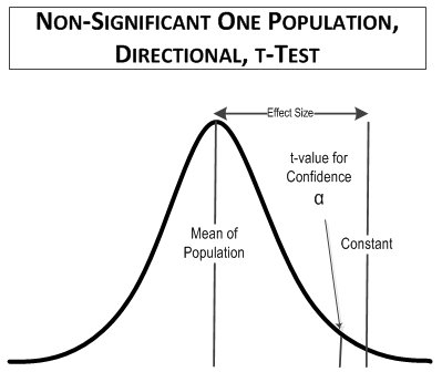
| Effect Size | The smallest difference the test could have detected. Effect size is influenced by the variance, the sample size, and the confidence. Effect size can be too small, leading to false negatives, or too large, leading to false positives. |
| Significance | Significance refers to the result of a statistical test in which the null hypothesis is rejected. Significance is expressed as a p-value. |
| Meaningfulness | Meaningfulness is assessed by considering the difference detected by the test to what magnitude of difference would be important in reality. |

Normal Distributions
After defining the population, the phenomena, and the test hypotheses, you measure the phenomenon on an appropriate number of individuals in the population. These measurements need to be independent of each other and representative of the population. Then, you need to assess whether it’s safe to assume that the frequency distribution of the measurements is similar to a Normal distributed. If it is, a z-test or a t-test would be in order.


| Yes, this is scary looking. It’s the equation for the Normal distribution. Relax, you will probably never have to use it. |
This figure represents a Normal distribution. The area under the curve represents the total probability of measured values occurring, which is equal to 1.0. Values near the center of the distribution, near the mean, have a large probability of occurring while values near the tails (the extremes) of the distribution have a small probability of occurring.
In statistical testing, the Normal distribution is used to estimate the probability that the measurements of the phenomenon will fall within a particular range of values. To estimate the probability that a measurement will occur, you could use the values of the mean and the standard deviation in the formula for the Normal distribution. Actually though, you never have to do that because there are tables for the Normal distribution and the t-distribution. Even easier, the functions are available in many spreadsheet applications, like Microsoft Excel.
Statistical tests focus on the tails of the distribution where the probabilities are the smallest. It doesn’t matter much if the measurements of the phenomenon follow a normal distribution near the mean so long as it does in the tails. The z-distribution can be used if the sample size is large; some say as few as 30 measurements and others recommend more, perhaps 100 measurements. The t-distribution compensates for small sample sizes by having more area in the tails. It can be used instead of the z-distribution with any number of samples.
The concept behind statistical testing is to determine how likely it is that a difference in two populations parameters like the means (or a population parameter and a constant) could have occurred by chance. If the probability of the difference occurring is large enough to occur in the tails of the distribution, there is only a small probability that the difference could have occurred by chance. Differences having a probability of occurrence less then a pre-specified value (α) are said to be significant differences. The pre-specified value, which is the acceptable false positive error rate, α, may be any small percentage but is usually taken as five-in-a-hundred (0.05), one-in-a-hundred (0.01), or ten-in-a-hundred (0.10).
Here are a few examples of what the process of statistical testing looks like for comparing a population mean to a constant.

One Population z-Test or t-Test
All z-tests and t-tests involve either one or two populations and only one phenomenon. The population is represented by the nominal-scale, independent variable. The measurement of the phenomenon is the dependent variable, which can be measured using a nominal, ordinal, interval, or ratio scale.
For a one-population test, you would be comparing the average (or other parameter) of the measurements in the population to a constant. You do this using the formula for a one-population t-test value (or a z-test value) to calculate the t value for the test.
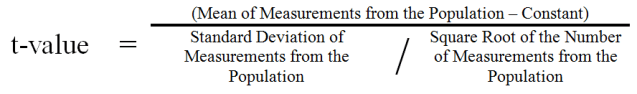
The Normal distribution and the t-distribution are symmetrical so it doesn’t matter if the numerator of the equation is positive or negative.
Then compare that value to a table of values for the t-distribution (for the appropriate number of tails, the confidence (1- α), and the degrees of freedom (the number of samples of the population minus 1). If the calculated t value is larger than the table t value, the test is SIGNIFICANT, meaning that the mean and the constant are statistically different. If the table t value is larger than the calculated t value, the test is NOT SIGNIFICANT, meaning that the mean and the constant are statistically the same.
Example
Imagine you are comparing the average height of male, high school freshmen, in Minneapolis school district #1. You want to know how their average height compares to the height of 9th to 11th century Vikings (their mascot), for the school newspaper. Turn-of-the-century Vikings were typically about 5’9” or 69 inches (172 cm) tall.
This comparison doesn’t need to be too rigorous. The only possible negative consequence to the test is it being reported by Fox News as a liberal conspiracy, and they do that to everything anyway. You’ll accept a false positive rate (i.e., 1-confidence, α) of 0.10.
Nondirectional Tests
Say you don’t know many freshmen boys but you don’t think they are as tall as Vikings. You certainly don’t think of them as rampaging Vikings. They’re younger so maybe they’re shorter. Then again, they’ve grown up having better diets and medical care so maybe they’re taller. Therefore, your research hypothesis is that Freshmen are not likely to be the same height as Vikings. The null hypothesis you want to test is:
Height of Freshmen = Height of Vikings
which is a nondirectional test. If you reject the null hypothesis, the alternative hypothesis:
Height of Freshmen ≠ Height of Vikings
is probably true of the Freshmen. Say you then measure the heights of 10 freshmen and you get:
63.2, 63.8, 72.8, 56.9, 75.2, 70.8, 68.0, 64.0, 61.4, 65.2
The measurements average 66 inches with a standard deviation of 5.3 inches. The t-value would be equal to:
(Freshmen height – Viking height) / ((standard deviation / (√number of samples)))
t-value = (66 inches – 69 inches) / (5.3 inches / (√10 samples))
t-value = -1.790
Ignore the negative sign; it won’t matter.
In this comparison, the calculated t-value (1.79) is less than the table t-value (t(2-tailed, 90% confidence, 9 degrees of freedom) = 1.833) so the comparison is not significant. The comparison might look something like this:
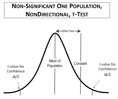
There is no statistical difference in the average heights of Freshmen and Vikings. Both are around 5’6” to 5’9” tall. That isn’t to say that there weren’t 6’0” Vikings, or Freshmen, but as a group, the Freshmen are about the same height as a band of berserkers. I’m sure that there are high school principals who will agree with this.
When you get a nonsignificant test, it’s a good practice to conduct a power analysis to determine what protection you had against false negatives. For a t-test, this involves rearranging the t-test formula to solve for tbeta:
tbeta = (sqrt(n)/sd) * difference – talpha
The talpha is for the confidence you selected, in this case 90%. Then you look up the t-value you calculated to find the probability for beta. It’s a cumbersome but not difficult procedure. In this example, the calculated tbeta would have been 1.24 so the power would have been 88%. That’s not bad. Anything over 80% is usually considered acceptable.
Most statistical software will do this calculation for you. You can increase power by increasing the sample size or the acceptable Type 1 error rate (decrease the confidence) before conducting the test.
So if everything were the same (i.e., mean of students = 66 inches, standard deviation = 5.3 inches) except that you had collected 30 samples instead of 10 samples:
t-value = (69 inches – 66 inches) / (5.3 inches / (√30 samples))
t-value = 3.10
t(2-tailed, 90% confidence, 29 degrees of freedom) = 1.699
If you had collected 100 samples:
t-value = (69 inches – 66 inches) / (5.3 inches / (√100 samples))
t-value = 5.66
t(2-tailed, 90% confidence, 99 degrees of freedom) = 1.660
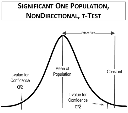
These comparisons are both significant, and might look something like this:
More samples give you better resolution.

Directional Tests
Now say, in a different reality, you know that many of those freshmen boys grew up on farms and they’re pretty buff. You even think that they might just be taller than the Vikings of a millennia ago. Therefore, your research hypothesis is that Freshmen are likely to be taller than the warfaring Vikings. The null hypothesis you want to test is:
Height of Freshmen ≤ Height of Vikings
which is a directional test. If you reject the null hypothesis, the alternative hypothesis:
Height of Freshmen >Height of Vikings
is probably true of the Freshmen. Then you measure the heights of 10 freshmen and get:
72.4, 71.1, 75.4, 69.0, 75.7, 73.3, 76.0, 58.8, 70.4, 78.6
The measurements average 71.2 inches with a standard deviation of 5.3 inches. The t-value would be equal to:
(Freshmen height – Viking height) / (standard deviation / (√number of samples))
t-value = (72 inches – 69 inches) / (5.3 inches / (√10 samples))
t-value = 1.790
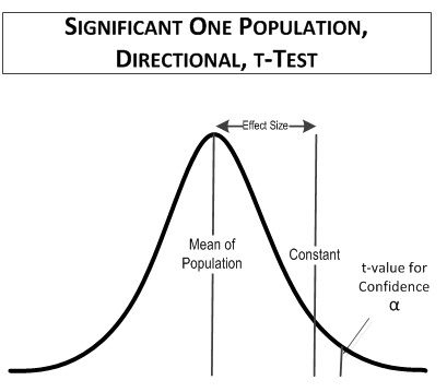
 In this comparison, the table t-value you would use is for a one-tailed (directional) test at 90% confidence for 10 samples, t(1-tailed, α = 0.1, 9 degrees of freedom) = 1.383. For comparison, the value of t(2-tailed, 0.9 confidence, 9 degrees of freedom), which was used in the first example, is equal to 1.833, as is t(1-tailed, 0.95 confidence, 9 degrees of freedom). The reason is that you only have to look in half of the t-distribution area in a one-tailed test compared to a two-tailed test. That means that if you use a directional test you can have a smaller false positive rate.
The table t value you would use, t(1-tailed, 0.1 confidence, 9 degrees of freedom), is equal to 1.383. which is smaller than the calculated t-value, 1.790, so the comparison is significant. The comparison might look something like this:
In this comparison, the Freshmen are on average at least 3 inches taller than their frenzied Viking ancestors. Genetics, better diet, and healthy living win out.
But what if the farm boys averaged only 71 inches:
(Freshmen height – Viking height) / (standard deviation / (√number of samples))
t-value = (71 inches – 69 inches) / (5.3 inches / (√10 samples))
t-value = 1.193
The table t value you would use, t(1-tailed, 0.1 confidence, 9 degrees of freedom), is equal to 1.383. which is larger than the calculated t-value, 1.193, so the comparison is not significant. The comparison might look something like this:
And that’s what one-population t-tests look like. Now for some two-population tests in Dare to Compare – Part 4.

Read more about using statistics at the Stats with Cats blog. Join other fans at the Stats with Cats Facebook group and the Stats with Cats Facebook page. Order Stats with Cats: The Domesticated Guide to Statistics, Models, Graphs, and Other Breeds of Data analysis at amazon.com, barnesandnoble.com, or other online booksellers.
 The American Statistical Association has identified
 Part 1 of Dare to Compare summarized several fundamental topics about statistical comparisons.
 Statistical tests that don’t rely on the distributions of the phenomenon in the populations are called nonparametric tests. Nonparametric tests often involve converting the data to ranks and analyzing the ranks using the median and the range.
 When you conduct a statistical test, the result does not mean you prove your hypothesis. Rather, you can only reject or fail to reject the null hypothesis. If you reject the null hypothesis, you adopt the alternative hypothesis. This would mean that it is more likely that the null hypothesis is not true in the populations. If you fail to reject the null hypothesis, it is more likely that the null hypothesis is true in the populations.
 After you conduct the test, there are two pieces of information you need to determine – the sensitivity of the test to detect differences, called the effect size, and the power of the test. The power of the test will depend on the sample size, the confidence, and the effect size. The effect size also provides insight into whether the test results are meaningful. Meaningfulness is important because a test may be able to detect a difference far smaller than what might of interest, such as a difference in mean student heights less than a millimeter. Perhaps surprisingly, the most common reason for being able to detect differences that are too small to be meaningful is having too large a sample size.
 z-Tests and t-Tests
 χ2 Tests
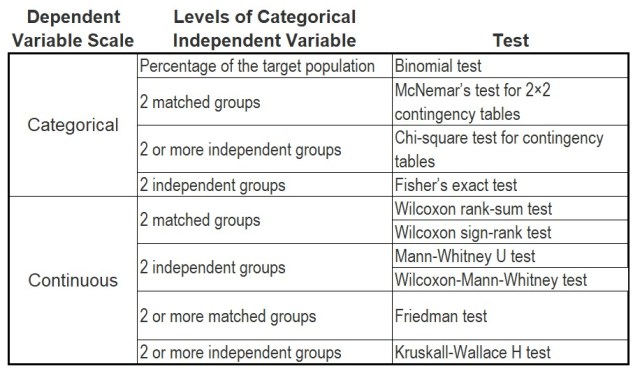

 In school, you probably had to line up by height now and then. That wasn’t too difficult. There weren’t too many individuals being lined up and they were all in the same place at the same time. An individual’s place in line was decided by comparing his or her height to the heights of other individuals. The comparisons were visual; no measurements were made. Everyone made the same decisions about the height comparisons. You didn’t need statistics to solve the problem. So why might you ever need statistics to compare heights?
 Fortunately, you don’t have to measure every individual in the population so long as you measure a representative sample of the individuals in the populations. You can improve your chances of getting a representative sample by using the three Rs of variance control —
  A bell curve is usually assumed to represent a Normal distribution. The average and the variance of the values are called parameters of the distribution because they are in the mathematical formula that defines the form of the distribution.
 Read more about using statistics at the
  Whether you know it or not, you deal with models every day. Your weather forecast comes from a meteorological model, usually several. Mannequins are used to display how fashions may look on you. Blueprints are drawn models of objects or structures to be built. Maps are models of the earth’s terrain. Examples are everywhere.
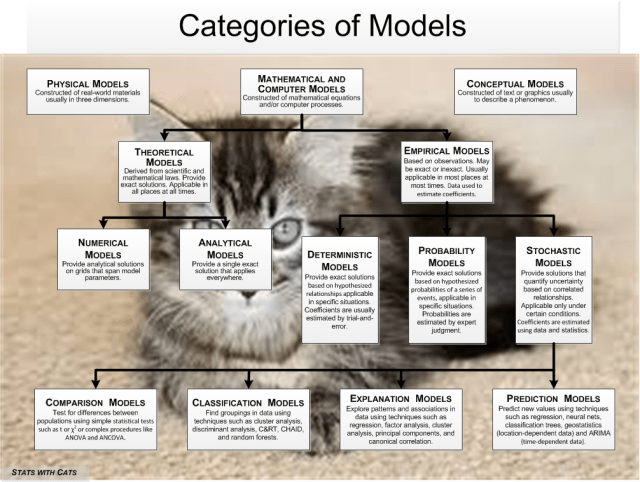

 Models can also be expressed in words and pictures. These are used in virtually all fields to convey mental images of some mechanism, process, or other phenomenon that was or will be created. Blueprints, flow diagrams, geologic fence diagrams, anatomical diagrams are all conceptual models. So are the textual descriptions that go with them. In fact, you should always start with a simple text model before you embark on building a complex physical or mathematical model.
 Theoretical Models
 Probability Models
 In statistical comparison models, the dependent variable is a grouping-scale variable (one measured on a nominal
  Clustering models do not have a nominal-scale dependent variable, but most classification models do.
  Factor Analysis
 Some models are created to predict new values of a dependent variable or forecast future values of a time-dependent variable. To be useful, a prediction model must use prediction variables that cost less to generate than the prediction is worth. So the predictor variables and their scales must be relatively inexpensive and easy to create or obtain. In prediction models, accuracy tends to come easy while precision is elusive. Prediction models usually keep only the variables that work best in making a prediction, and they may not necessarily make a lot of conceptual sense.
 Step 1 – Start at top of the Catalog of Models figure. Decide whether you want to create a physical, mathematical, or conceptual model. Whichever you choose, start by creating a brief conceptual model so you have a mental picture of what your ultimate goal is and can plan for how to get there.
 Say you wanted to describe someone you see on the street. You might characterize their sex, age, height, weight, build, complexion, face shape, hair, mouth and lips, eyes, nose, tattoos, scars, moles, and birthmarks. Then there’s clothing, behavior, and if you’re close enough, speech, odors, and personality. Your description might be different if you’re talking to a friend or a stranger, of the same or different sex and age. Those are a lot of characteristics and they’re sometimes hard to assess. Individual characteristics aren’t always relevant and can change over time. And yet, without even thinking about it, we describe people we see every day using these characteristics. We do it mentally to remember someone or overtly to describe a person to someone else. It becomes second nature because we do it all the time.


 Shape refers to the frequency of the values in a dataset at selected levels of the scale, most often depicted as a graph. For ordinal scales, the graph is usually a histogram. For continuous scales, the graph is usually a probability plot, although sometimes histograms are used. Shapes of continuous scale data can be compared to mathematical models (equations) of frequency distributions. It’s like comparing a person to some well-known celebrity; they’re not identical but are similar enough to provide a good comparison. There are dozens of such distribution models, but the most commonly used is the
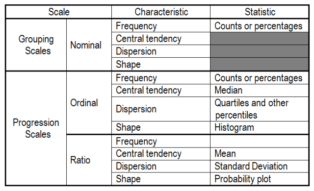


 -ended responses on surveys, social networking sites, email, online reviews, public comments, notations (e.g., medical, customer relations), documents and text files, or even recorded and transcribed interactions. But before anything can happen, you have to accomplish three tasks:
 e are several ways that you can
  ll want to aggregate them to make things easier. If you have text on a website, you can usually highlight it and copy it using <ctrl-C>. If the passage is long, you can use <ctrl-A> to select everything before copying it, but you’ll have to edit out the extraneous material. You can do these operations in most word processors.
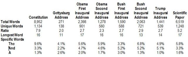

 Step 4 – Count the Fragments Assigned to Each Descriptor
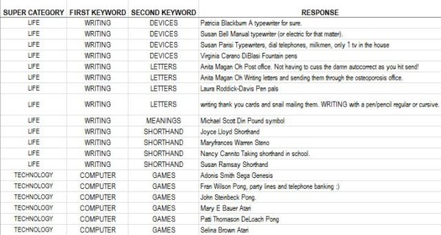

 Any variable that you record in a dataset will have some scale of measurement. Scales of measurement are, simply put, the ways that associated numbers relate to each other. Scales are properties of numbers, not the objects being measured. You could measure the same attribute of an object using more than one scale. For example, say you were doing a study involving cats and wanted to have a measure of each cat’s age. If you knew their actual birth dates, you could calculate their real ages in years, months, and days. If you didn’t know their birth dates, you could have a veterinarian or other knowledgeable individual estimate their ages in years. If you didn’t need even that level of precision, you could simply classify the cats as kittens, adult cats, or mature cats.
 In Statistics 101, you’ll learn that there are four types of measurement scales – nominal, ordinal, interval, and ratio. This isn’t entirely true. The four-scale classification, described by Stevens (1946)


 because the choice of sea level as the zero elevation is arbitrary. Time can also be thought of as an interval scale.

 poral trends. The third approach is used by statisticians who want to show off.

 nsional. Thus, coordinate systems usually have to be converted for one to the other. Geostatistical applications, for example, are based on distance and direction measurements but these measurements are calculated from spatial coordinates.
 r represent the progression in a variable’s attribute, whether simple, ordinal-scale levels or more expansive ratio-scale levels. One way to view these differences is this: nominal (grouping) scales are like stone outcrops, randomly scattered around a garden area. Ordinal scales are like garden steps. You can only be on a step not between steps, and the steps lead progressively upward or downward. There may be many steps or just a few. Ratio scales are like a garden path or ramp. You can be anywhere along the path, at high levels or low. You can move forward or back, in small or large intervals.
 a nominal scale. You can buy one of their cars painted red or blue or silver or black. To a gemologist, the color of a diamond is graded on an ordinal scale from D (colorless) to Z (light yellow). To an artist, color is measured on an interval scale because their color wheel contains the sequence: red, red-orange, orange, orange-yellow, yellow, yellow-green, green, green-blue, blue, blue-violet, violet, and violet-red. To a physicist, colors are measured by a continuous spectrum of light frequencies, which employ a ratio scale.
 w an ordinal scale could be applied. You can almost always devise an ordinal scale to characterize an attribute; you just have to be


