Reports vs. Analyses

Data reports are not the same as data analyses. It’s like with your checking account. Sometimes you just want a quick report of your balance. That information from the bank’s database has to be up-to-date and readily available when you need it. Reports may include all the data or just summaries and graphs. People looking at a report have to figure out what it means. If you want to figure out where you’re spending your money, you have to conduct an analysis. You’ll have to compile the data, scrub out anomalies, look for patterns, and interpret the results. People looking at an analysis have to figure out what to do with the information.

Reports = data + descriptive statistics and graphs

Analyses = data + number crunching + interpretation

Posted in Uncategorized | 2 Comments

Survey Avoidance Disorder

Posted in Uncategorized | Leave a comment

The Best Super Power of All

If you’re not a mutant, an extraterrestrial, an adventure seeker prone to outlandously fortuitous accidents, or a wealthy scientific genius who can engineer all sorts of wondrous gadgets, don’t despair. You can still have your own super power. In fact, it’s the best super power of all. It’s the power of critical thinking.

No human can resist my Super Cuteness.

What’s critical thinking? It’s simply being able to assess the truthfulness and validity of the things people say. That may not sound as awesome as super speed or morphing into an animal, but it has distinct advantages. With critical thinking, you don’t need a special costume. You don’t need to hide your power or protect your identity or explain why your clothes are torn apart. It won’t leave you physically exhausted and doesn’t involve fisticuffs (usually).

You can use critical thinking anywhere in any situation. You can use it on your teachers and classmates, your boss and co-workers, the trolls on Reddit, politicians and pundits, salesmen and ministers, and everyone else who tries to get into your head. And, you can learn to think critically whether you’re sixteen or sixty. All you have to do is to practice, but not grueling hours every day in the gym, just some easy mental exercises. Here’s how.

Stage 1 — Listen

Every super hero has a weakness; mine is catniptonite.

Start simply. Pay attention to the conversations you have, the internet forums you follow, the TV you watch, especially the ads, and any other communication you may read, watch, or hear. Then, decide if the communication is meant to persuade you to do or think something. If it doesn’t, ignore it for the time being. Focus on those communications that want you to buy a product, or accept a belief, or support a position. You need to be able to recognize these arguments at sight, almost without thinking. Take as long as you need to get good at this. Remember, it took Spiderman more than a few tries to learn to cling to walls, but if he hadn’t, he wouldn’t have been able to swing from building to building.

Stage 2 — Parse

Once you can easily identify those attempts to persuade you, the next step is to pick apart the pieces of those arguments. Think of arguments as consisting of three parts:

  • Premises — the facts the argument relies on
  • Logic — the way the premises are manipulated
  • Conclusion — the result of the argument.

You need to learn to identify these pieces before you can start evaluating the validity of an argument. This process wouldn’t be difficult if you only talked to other critical thinkers. Unfortunately, most people aren’t critical thinkers and the torrent of mental chaos you’ll encounter from them is daunting. So again, start simply. Look up examples of formal arguments on Wikipedia and then other Internet and textbook sources. When you’re comfortable with picking out the parts of formal arguments, you can move on to the chaotic musings of the idiocracy. In those, you’ll find more of a challenge. The parts of those arguments don’t always come in the customary premise-logic-conclusion order. Some arguments don’t spell out all the premises. The logic behind arguments is often unstated. The conclusion is the only thing you can count on being present, but it may be the first, and sometimes, the only part of an argument you’ll hear. With practice, you’ll get good at it. And when you do, you’ll find that, even at this point, you are developing a greater awareness of critical thought than most of your cohorts.

Stage 3 — Check

This is where learning to think critically gets interesting. Stage 3 involves looking at the components of arguments, which you should now be really good at picking out, and checking them for common flaws. Here are some things you should look for:

  • Premises — Are the premises actual facts or just someone’s claim? The argument may or may not cite a source, but even if it does, that doesn’t always mean the fact is valid. Sometimes a source is biased or just a regurgitation of another biased source. Get into the habit of searching the internet for verification. Start with relatively unbiased sites like snopes.com, factcheck.org, and procon.org, then start looking at other sites. You’ll develop a feel for the biased sites and how they spin information. Before long, you’ll find you’re developing a highly capable bullcrap detector that’s even better than Spidy sense.

Captain America’s shield is no match for my hairball missiles.

  • Logic – Don’t worry too much at this point about whether the logic is correct. Instead, look for obviously incorrect logic indicated by the presence of any of the most common fallacies. There are dozens of different fallacies, so start with these, which are usually easy to spot:

Judgmental language, making an argument using emotion-laden words. Phrases like religious fanatics, free-loading welfare recipients, lazy unemployed, and greedy bankers all impart more than just the essence of the argument. In today’s contentious society, judgmental language is hard not to find.

Ad hominum, an attack on the opponent rather than the opponent’s position. This happens all the time on political forums and often involves a reference to Hitler, illegal activities involving animals, or body parts.

Appeal to false authority, basing an argument on someone who isn’t really an expert, like all those celebrities on infomercials. Avoid peer pressure and the hive mind; think for yourself. Also beware of any reliance on common sense, which is more myth than magic.

After you are comfortable with these fallacies, visit Wikipedia and read about others like straw man, cherry picking, red herring, oversimplication, begging the question, slippery slope, equivocation, and quoting out of context. Take them one step at a time.

I have more claws than Wolverine and I know how to use them.

  • Conclusion – Argument conclusions can be of two types. Deductive arguments use premises about general information to conclude something specific. Sherlock Holmes, Doctor Who, and Patrick Jane (The Mentalist) are all masters of deduction, albeit fictional. Inductive arguments use premises about specific information to conclude something general. Beware of inductive arguments based on anecdotes, like Ronald Reagan’s legendary welfare queen. Induction usually involves statistics and probability because counterexamples are such easy argument killers, in which case it’s called abductive reasoning. Other than anecdotes, settle for being able to distinguish the two basic types of arguments.

The point of this stage is for you to be able to identify the more obvious red flags. If you complete this stage, you will be far ahead of most people. Enjoy your mental prowess and use it every day.

Stage 4 — Triage

I’m Catman.

You’ll find that you can spot a lot of faulty arguments just by knowing these few things to look for. In fact, you’ll probably find most of the arguments you listen to are faulty in one way or another. And that’s the problem. You have to be judicious with how you use your new power to think critically. You can’t just engage in battle with every troll who wants to argue over a movie, or a quarterback, or worst of all, a politician. Still, with great power comes great responsibility. You have to slap down some arguments. Given that, you’ll need to develop a sense for when you have tostep up to expose idiocy and when you can roll your eyes and let it slide. Further, you’ll have to develop a sense for when you have inflicted enough damage to withdraw. Heroes don’t slaughter their enemies; humiliation works just as well. You must become a guerrilla thinker. Pick your battles. Fight them in earnest. Then dissolve into the shadows. This is harder to do than it seems.

Stage 5 — Analyze

Most deciples of critical thinking get at least as far as stage 4. Elite thinkers go far beyond that to thoroughly analyzing all the components of an argument. Analyzing arguments is challenging. It requires knowledge of a broad variety of subjects, the development of sophisticated analytical skills like statistics and logic, the availability of resources that can support your quest for the truth, and lots and lots of practice. This learning process never ends. The more you know the more sophisticated are the arguments you’ll take on.

Here are some of the things you might explore to become an elite thinker.

  • Premises — Indisputable facts make good premises but not all facts are indisputable. Some premises purported to be facts are actually opinions or factoids (i.e, assertions that are made so commonly that they are assumed to be true). Elite thinkers also do not just consider the source of the fact because facts from even obstentiously unbiased, primary sources may not be entirely valid. Data analysis can be idiosyncratic. For example, different statisticians may come to different conclusions from the same data set because of the way they scrub the data, transform variables, and conduct analyses. Another sign of an invalid data analyses is a lack of reference points like baselines and control groups. There are many other red flags that elite thinkers know to look for. In time, so can you.
  • Logic — There are many more fallacies that you can learn to recognize, though you’ll probably have to read textbooks to go beyond the easy pickings found on the Internet. But elite thinkers don’t just look for errors (fallacies), they also consider the proper use of logical processes, the rules used to convert premises into conclusions. In deductive reasoning, these logical processes are called propositional logicrules. For example, using the letters P, Q, and R for premises:
    • If P entails Q and P is true then Q is also true (called Modus Ponens)
    • If P entails Q and Q is false then P is also false (called Modus Tollens)
    • If P entails Q and Q entails R then P entails R (called Hypothetical Syllogism).

I am a Time Lord. I can sleep 18 hours a day and still know when to wake you up for gooshy food.

As you might guess, there are many more logical rules. Presumably, this is what Spock spent all those years studying on Vulcan. For inductive reasoning, an appreciation of statistical thinking is required. In essence, statistical thinking posits that everything is connected, everything has an inherent and extraneous variability, and extraneous variability needs to be controlled. Fatal flaws in inductive arguments usually stem from a failure to understand these concepts.

  • Conclusions — For any critical thinker, the validity of an argument is paramount, but for elite thinkers, the subtleties of how an argument is presented is also important. This is where having a good understanding of modes of communication, writing styles, propaganda, pragmatic context, and subliminal and nonverbal communications are essential.

So there is the path to becoming a critical thinker. Getting started isn’t difficult, it just takes practice. The more you practice the more you’ll learn. The more you learn the better you’ll be at it. Just give it a try. Once you start experiencing the rewards, you’ll understand why critical thinking is the best super power of all.

This blog is dedicated to Alex Finkel, my friend Ray Finkel’s nephew, and to all the other graduates of 2012. Strive to make this world better for everyone.

Read more about using statistics at the Stats with Cats blog. Join other fans at the Stats with Cats Facebook group and the Stats with Cats Facebook page. Order Stats with Cats: The Domesticated Guide to Statistics, Models, Graphs, and Other Breeds of Data Analysis at Wheatmarkamazon.combarnesandnoble.com, or other online booksellers.

Posted in Uncategorized | Tagged , , , | 16 Comments

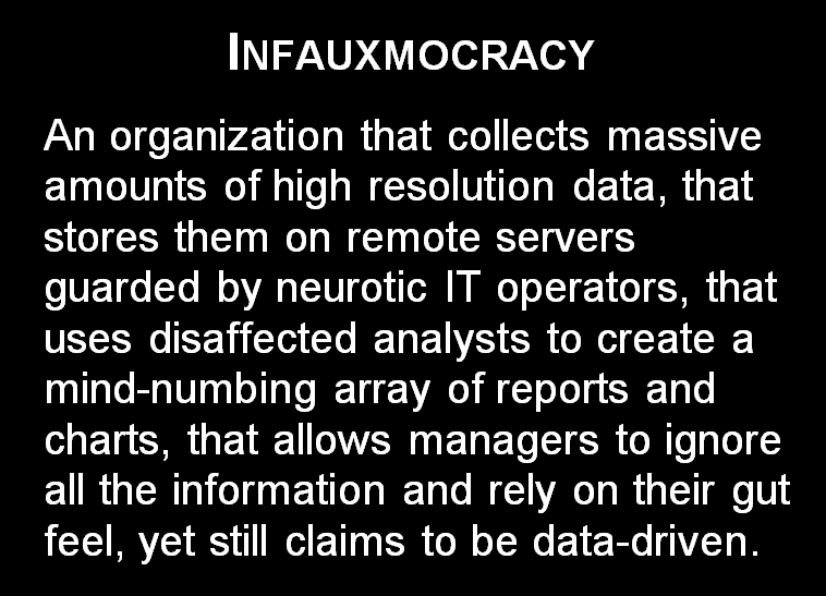
Infauxmocracy

Posted in Uncategorized | 2 Comments

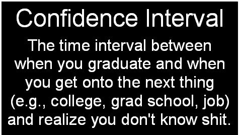
Confidence Interval

Posted in Uncategorized | Leave a comment

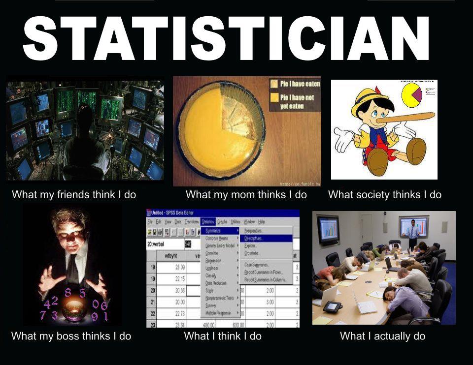
What Does a Statistician Do

This is what people think I do.

Posted in Uncategorized | 9 Comments

Five Things You Should Know Before Taking Statistics 101

I can’t wait to take Statistics 101 now that I know this stuff.

Of the over two million college degrees that are granted in the U.S. every year, including those earned at accredited online colleges nationwide, probably two-thirds require completion of a statistics class. That’s over a million and a half students taking Statistics 101, even more when you consider that some don’t complete the course.

Everybody who has completed high school has learned some statistics. There are good reasons for that. Your class grades were averages of scores you received for tests and other efforts. Most of your classes were graded on a curve, requiring the concepts of the Normal distribution, standard deviations, and confidence limits. Your scores on standardized tests, like the SAT, were presented in percentiles. You learned about pie and bar charts, scatter plots, and maybe other ways to display data. You might even have learned about equations for lines and some elementary curves. So by the time you got to prom, you were exposed to at least enough statistics to read USA Today.

Faced with taking Statistics 101, you may be filled with excitement, ambivalence, trepidation, or just plain terror. Your instructor may intensify those feelings with his or her teaching style and class requirements. So to make things just a bit easier, here are a few concepts to remember.

Everything is Uncertain

The fundamental difference between statistics and most other types of data analysis is that in statistics, everything is uncertain. Input data have variabilities associated with them. If they don’t, they are of no interest. As a consequence, results are always expressed in terms of probabilities.

Every data measurement is variable, consisting of:

  • Characteristic of Population—This is the part of a data value that you would measure if there were no variability. It’s the portion of a data value that is the same between a sample and the population the sample if from.
  • Natural Variability—This part of a data value is the uncertainty or variability in population patterns. It’s the inherent differences between a sample and the population. In a completely deterministic world, there would be no natural variability.
  • Sampling Variability—This is the difference between a sample and the population that is attributable to how uncharacteristic (non-representative) the sample is of the population.
  • Measurement Variability—This is the difference between a sample and the population that is attributable to how data were measured or otherwise generated.
  • Environmental Variability— This is the difference between a sample and the population that is attributable to extraneous factors.

The goal of most statistical procedures is to estimate the characteristic of the population, characterize the natural variability, and control and minimize the sampling, measurement, and environmental variability. Minimizing variance can be difficult because there are so many causes and because the causes are often impossible to anticipate or control. So if you’re going to conduct a statistical analysis, you’ll need to understand the three fundamentals of variance control—Reference, Replication, and Randomization.

Statistics Models

Statistics and models are closely intertwined. Models serve as both inputs and outputs of statistical analyses. Statistical analyses begin and end with models.

Statistics uses distribution models (equations) to describe what a data frequency would look like if it were a perfect representation of the population. If data follow a particular distribution model, like the Normal distribution, the model can be used as a template for the data to represent data frequencies and error rates. This is the basis of parametric statistics; you evaluate your data as if they came from a population described by the model.

Statistical techniques are also used to build models from data. Statistical analyses estimate the mathematical coefficients (parameters) for the terms (variables) in the model, and include an error term to incorporate the effects of variation. The resulting statistical model, then, provides an estimate of the measure being modeled along with the probability that the model might have occurred by chance, based on the distribution model.

Measurement Scales shape Analyses

You may not hear very much about measurement scales in Statistics 101, but you should at least be aware of the difference between nominal scales, ordinal scales, and continuous scales. Nominal scales, also called grouping or categorical scales, are like stepping stones; each value of the scale is different from other values, but neither higher nor lower. Discrete scales are like steps; each value of the scale has a distinct break from the next discrete value, which is either higher or lower. Continuous scales are like ramps; each value of the scale is just a little bit higher or lower than the next value. There are many more types of scales, especially for time scales, but that’s enough for Statistics 101.

The reason measurement scales are important is that they will help guide which graph or statistical procedure is most appropriate for an analysis. In some situations, you can’t even conduct a particular statistical procedure if the data scales are not appropriate.

Everything Starts with a Matrix

You may not realize it in Statistics 101, but all statistical procedures involve a matrix. Matrices are convenient ways to assemble data so that computers can perform mathematical calculations. If you go beyond Statistics 101, you’ll learn a lot about matrix algebra. But for Statistics 101, all you have to know is that a matrix is very much like a spreadsheet. In a spreadsheet you have rows and columns that define rectangular areas, called cells. In statistics, the rows of the spreadsheet represent individual samples, cases, records, observations, entities that you’re making measurements on, sample collection points, survey respondents, organisms, or any other point or object on which information is collected. The columns represent variables, the measurements or the conditions or the types of information you’re recording. The columns can correspond to instrument readings, survey responses, biological parameters, meteorological data, economic or business measures, or any other types of information. You usually have several sets of variables for a given set of samples. Together, the rows and the columns of the spreadsheet define the cells, which is where the data are stored. Samples (rows), variables (columns), and data (cells) are the matrix that goes into a statistical analysis. If you understand data matrices, you’ll be able to conduct statistical analyses even without your Statistics 101 instructor to help you.

Statistics is More than Description and Testing

In Statistics 101, you learn about probability, distribution models, populations, and samples. Eventually, this knowledge will enable you to be able to describe the statistical properties of a population and to test the population for differences from other populations. But these capabilities, formidable though they are, don’t reveal the truly mind boggling analyses you can do with statistics. You can:

  • Describe—characterizing populations and samples using descriptive statistics, statistical intervals, correlation coefficients, and graphics.
  • Compare and Test—detecting differences between statistical populations or reference values using simple hypothesis tests, and analysis of variance and covariance.
  • Identify and Classify—identifying known or hypothesized entities or classifying groups of entities using descriptive statistics; statistical tests, graphics, and multivariate techniques such as cluster analysis and data mining techniques.
  • Predict—predicting measurements using regression and neural networks, forecasting using time-series modeling techniques, and interpolating spatial data.
  • Explain—explaining latent aspects of phenomena using regression, cluster analysis, discriminant analysis, factor analysis, and other data mining techniques.

So don’t get discouraged if you can’t see how statistics will help you in your career based on Statistics 101. There’s a lot more out there. You just have to take the first step.

Read more about using statistics at the Stats with Cats blog. Join other fans at the Stats with Cats Facebook group and the Stats with Cats Facebook page. Order Stats with Cats: The Domesticated Guide to Statistics, Models, Graphs, and Other Breeds of Data Analysis at Wheatmark, amazon.combarnesandnoble.com, or other online booksellers.
Posted in Uncategorized | Tagged , , , , , , , , , , , , , , | 24 Comments

Polls Apart

Election season is fast approaching so you can be sure a plethora of polls will soon be adding to the mayhem. Polls educate us in two ways. They tell us what we, or at least the population being polled, think. And, in a more Orwellian sense, they tell us what we should think. Polls are used to guide how the nation is governed. For example, did you know that the unemployment rate is determined from a poll, called the Current Population Survey? Polls are important, so we need to be enlightened consumers of poll results lest we come to “love Big Brother.”

The growth of polling has been exponential, following the evolution of the computer and statistical software. Before 1990, the Gallup Organization was pretty much the only organization conducting presidential approval polls. Now, there are several dozen. On average, there were only one or two presidential approval polls conducted per month. Within a decade, that number had increased to more than a dozen. These pollsters don’t just ask about Presidential approval, either. Polls are conducted on every issue of real importance and most of the issues of contrived importance. Many of these polls are repeated to look for changes in opinions over time, between locations, and for different demographics. And that’s just political polls. There has been an even faster increase in polling for marketing, product development, and other business applications.

So to be an educated consumer of poll information, the first thing you have to recognize is which polls should be taken seriously. Forget internet polls. Forget polls conducted in the street by someone carrying a microphone. Forget polls conducted by politicians or special-interest groups. Forget polls not conducted by a trained pollster with a reputation to protect.

For the polls that remain, consider these four factors:

  • Difference between the choices
  • Margin of error
  • Sampling error
  • Measurement error

Here’s what to look for.

Difference between Choices

The percent difference between the choices on a survey is often the only thing people look at, with good reason. It is often the only thing that gets reported. Reputable pollsters will always report their sample size, their methods, and even their poll questions, but that doesn’t mean all the news agencies, bloggers, and other people who cite the information will do the same. But the percent difference between the choices means nothing without also knowing the margin-of-error. Remember this. For any poll question involving two choices, such as Option A versus Option B, the largest margin of error will be near a 50%–50% split. Unfortunately, that’s where the difference is most interesting, so you really need to know something about the actual margin of error.

Margin-of-Error

You might have seen surveys report that the percent difference between the choices for a question has a margin-of-error of plus-or-minus some number. In fact, the margin-of-error describes a confidence interval. If survey respondents selected Option A 60% of the time with a margin-of-error of 4%, the actual percentage in the sampled population would be 60% ± 4%, meaning between 56% and 64%, with some level of confidence, usually 95%.

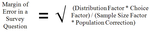
For a simple random sample from a surveyed population, the margin-of-error is equal to the square root of a Distribution Factor times a Choice Factor divided by a Sample Size Factor times a Population Correction.

  • Distribution Factor is the square of the two-sided t-value based on the number of survey respondents and the desired confidence level. The greater the confidence the larger the t-value and the wider the margin-of-error.
  • Choice Factor is the percentage for Option A times the percentage for Option B. That’s why the largest margin of error will always be near a 50%–50% split (e.g., 50% times 50% will always be greater than any other percentage split, like 90% times 10%).
  • Sample Size Factor is the number of people surveyed. The more people you survey, the smaller the margin of error.
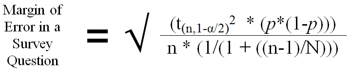
  • Population Correction is an adjustment made to account for how much of a population is being sampled. If you sample a large percentage of the population, the margin-of-error will be smaller. The population correction ranges from 1 to about 2. It is calculated by the reciprocal of one plus the quantity the number of people surveyed (n) minus one divided by the number of people in the population (N), or in mathematical notation, 1/(1+(n-1/N)).

So the entire equation for the margin-of-error is:

Or in mathematical notation:


This formula can be simplified by making a few assumptions.

  1. If the population size (N) is large compared to the sample size (n), you can ignore the Population Correction. What’s large, you ask? A good rule of thumb is to use the correction if the sample size is more than 5% of the population size. If you’re conducting a census, a survey of all individuals in a population, you can’t make this assumption.
  2. Unless you expect a different result, you can assume the percentages for respondent choices will be about 50%–50%. This will provide the maximum estimate for the margin-of-error, ignoring other factors.
  3. Ignore the sample size in the Distribution Factor and use a z-score instead of a t-score. For a two-sided margin-of-error having 95% confidence, the z-score would be 1.96.
  4. The Distribution Factor (1.962) times the Choice Factor (50%2) equals 0.96

These assumptions reduce the equation for the margin-of-error to 1/n. What could be simpler? Here’s a chart to illustrate the relationship between the number of responses and the margin-of-error. The margin-of-error gets smaller with an increase in the number of respondents, but the decrease in the error becomes smaller as the number of responses increases. Most pollsters don’t use more than about 1,200 responses simply because the cost of obtaining more responses isn’t worth the small reduction in the margin-of-error. Don’t worry about the Current Population Survey, though. The Bureau of Labor Statistics polls about 110,000 people every month so their margin-of-error is less than half of a percentage point.

Always look for the margin-of-error to be reported. If it’s not, look for the number of survey responses and use the chart or the equation to estimate the margin of error. Here’s a good point of reference. For 1,000 responses, the margin-of-error will be about ±3% for 95% confidence. So if a political poll indicates that your candidate is behind by two points, don’t panic; the election is still too close to call.

Sampling Error

Sampling error in a survey involves how respondents are selected. You almost never see this information reported about a survey for several reasons. First, it’s boring unless you’re really into the mechanics of surveys. Second, some pollsters consider it a trade secret that they don’t want their competition to know about especially if they’re using some innovative technique to minimize extraneous variation. Third, pollsters don’t want everyone to know exactly what they did because then it might become easy to find holes in the analysis.

Ideally, potential respondents would be selected randomly from the entire population of respondents. But you never know who all the individuals are in a population, so have to use a frame to access the individuals who are appropriate for your survey. A frame might be a telephone book, voter registration rolls, or a top-secret list purchased from companies who create lists for pollsters. Even a frame can be problematical. For instance, to survey voter preferences a list of registered voters would be better than a telephone book because not everyone is registered to vote. But even a list of registered voters would not indicate who will actually be voting on Election Day. Bad weather might keep some people at home while voter assistance drives might increase turnout of a certain demographic.

A famous example of a sampling error occurred in 1948 when pollsters conducted a telephone survey and predicted that Thomas E. Dewey would defeat Harry S. Truman. At the time, telephones were a luxury owned primarily by the wealthy, who supported Dewey. When voters, both rich and poor, went to the polls, it was Truman who was victorious. This may seem obvious in retrospect but there’s an analogous issue today. When cell phones were introduced, the numbers were not compiled into lists, so cell phone users, primarily younger individuals, were under sampled in surveys conducted over land lines.

Another issue is that survey respondents need to be selected randomly from a frame by the pollster to ensure that bias is not introduced into the study. Open-invitation internet surveys fail to meet this requirement, so you can never be sure if the survey has been biased by freepers. Likewise, if someone with a microphone approaches you on the street it’s more likely to be a late night talk show host than a legitimate pollster.

Measurement Error

Measurement error in a survey usually involves either the content of a survey or the implementation of the survey. You might get to see the survey questions but you’ll never be able to assess the validity of the way a survey is conducted.

Content involves what is asked and how the question is worded. For example, you might be asked “what is the most important issue facing our country” with the possible responses being flag burning, abortion, social security, Congressional term limits, or earmarks. Forget unemployment, the economy, wars, education, the environment, and everything else. You’re given limited choices so that other issues can be reported to be less important.

Politicians are notorious for asking poll questions in ways that will support their agenda. They also use polls not to collect information but to dissemination information about themselves or disinformation about their opponents. This is called push polling.

The last thing to think about for a poll is how the responses were collected. For autonomous surveys, look at how the questions are worded. For direct response surveys, even if you could get a copy of the script used to ask the questions, there’s no telling what was actually said, what body language was used, and so on. Professional pollsters may create the surveys but they are often implemented by minimally trained individuals.


Read more about using statistics at the Stats with Cats blog. Join other fans at the Stats with Cats Facebook group and the Stats with Cats Facebook page. Order Stats with Cats: The Domesticated Guide to Statistics, Models, Graphs, and Other Breeds of Data Analysis at Wheatmark, amazon.combarnesandnoble.com, or other online booksellers.


Posted in Uncategorized | Tagged , , , , , , , , , , , | 4 Comments

Regression Fantasies: Part III

Is Your Regression Model Telling the Truth?

I’ve looked at your model and I’m afraid I have some bad news for you.

There are many technologies we use in our lives without really understanding how they work. Television. Computers. Cell phones. Microwave ovens. Cars. Even many things about the human body are not well understood. But I don’t mean how to use these mechanisms. Everyone knows how to use these things. I mean understanding them well enough to fix them when they break. Regression analysis is like that too. Only with regression analysis, sometimes you can’t even tell if there’s something wrong without consulting an expert.

Here are some tips for troubleshooting regression models.

Diagnosis

You may know how to use regression analysis, but unless you’re an expert, you may not know about some of the more subtle pitfalls you may encounter. The biggest red flag that something is amiss is the TGTBT, too good to be true. If you encounter an R-squared value above 0.9, especially unexpectedly, there’s probably something wrong. Another red flag is inconsistency. If estimates of the model’s parameters change between data sets, there’s probably something wrong. And if predictions from the model are less accurate or precise than you expected, there’s probably something wrong. Here are some guidelines for troubleshooting a model you developed.

Your Model

Identification

Correction

Not Enough Samples If you have fewer than 10 observations for each independent variable you want to put in a model, you don’t have enough samples. Collect more samples. 100 observations per variable is a good target to shoot for although more is usually better.
No Intercept You’ll know it if you do it. Put in an intercept and see if the model changes.
Stepwise Regression You’ll know it if you do it. Don’t abdicate model building decisions to software alone.
Outliers Plot the dependent variable against each independent variable. If more than about 5% of the data pairs plot noticeable apart from the rest of the data points, you may have outliers. Conduct a test on the aberrant data points to determine if they are statistical anomalies. Use diagnostic statistics like leverage to evaluate the effects of suspected outliers. Evaluate the metadata of the samples to determine if they are representative of the population being modeled. If so, retain the outlier as an influential observation (AKA leverage point).
Non-linear relationships Plot the dependent variable against each independent variable. Look for nonlinear patterns in the data Find an appropriate transformation of the independent variable.
Overfitting If you have a large number of independent variables, especially if they use a variety of transformation and don’t contribute much to the accuracy and precision of the model, you may have overfit the model. Keep the model as simple as possible. Make sure the ratio of observations to independent variables is large. Use diagnostic statistics like AIC and BIC to help select an appropriate number of variables.
Misspecification Look for any variants of the dependent variable in the independent variables. Assess whether the model meets the objectives of the effort. Remove any elements of the dependent variable from the independent variables. Remove at least one component of variables describing mixtures. Ensure the model meets the objectives of the effort with the desired accuracy and precision..
Multicollinearity Calculate correlation coefficients and plot the relationships between all the independent variables in the model. Look for high correlations. Use diagnostic statistics like VIF to evaluate the effects of suspected multicollinearity. Remove intercorrelated independent variables from the model.
Heteroscedasticity Plot the variance at each level of an ordinal-scale dependent variable or appropriate ranges of a continuous-scale dependent variable. Look for any differences in the variances of more than about five times. Try to find an appropriate Box-Cox transformation or consider nonparametric regression or data mining methods.
Autocorrelation Plot the data over time, location or the order of sample collection. Calculate a Durbin–Watson statistic for serial correlation. If the autocorrelation is related to time, develop a correlogram and a partial correlogram. If the autocorrelation is spatial, develop a variogram. If the autocorrelation is related to the order of sample collection, examine metadata to try to identify a cause.
Weighting You’ll know it if you do it. Compare the weighted model with the corresponding unweighted model to assess the effects of weighting. Consider the validity of weighting; seek expert advice if needed.

Sometimes the model you are skeptical about isn’t one you developed; it is models that are developed by other data analysts. The major difference is that with other analysts’ models, you won’t have access to all their diagnostic statistics and plots, let alone their data. If you have been retained to review another analyst’s work, you can always ask for the information you need. If, however, you’re reading about a model in a journal article, book, or website, you’ve probably got all the information you’re ever going to get. You have to be a statistical detective. Here are some clues you might look for.

Another Analyst’s Model

Identification

Not Enough Samples If the analyst reported the number of samples used, look for at least 10 observations for each independent variable in the model,
No Intercept If the analyst reported the actual model (some don’t), look for a constant term.
Stepwise Regression Unless another approach is reported, assume the analyst used some form of stepwise regression.
Outliers Assuming the analyst did not provide plots of the dependent variable versus the independent variables, look for R-squared values that are much higher or lower than expected.
Non-linear relationships Assuming the analyst did not provide plots of the dependent variable versus the independent variables, look for a lower-than- expected R-squared value from a linear model. If there are non-linear terms in the model, this is probably not an issue.
Overfitting Look for a large number of independent variables in the model, especially if they different types of transformation
Misspecification Look for any variants of the dependent variable in the independent variables. Assess whether the model meets the objectives of the effort.
Multicollinearity Assuming relevant plots and diagnostic statistics are not available, there may not be any way to identify multicollinearity.
Heteroscedasticity Assuming relevant plots and diagnostic statistics are not available, there may not be any way to identify heteroscedasticity.
Autocorrelation Assuming relevant plots and diagnostic statistics are not available, there may not be any way to identify serial correlation.
Weighting Compare the reported number of samples to the degrees of freedom. Any differences may be attributable to weighting.

No Doubts

So there are some ways you can identify and evaluate eleven reasons for doubting a regression model. Remember when evaluating other analyst’s models that not everyone is an expert and that even experts make mistakes. Try to be helpful in your critiques, but at a minimum, be professional.


Read more about using statistics at the Stats with Cats blog. Join other fans at the Stats with Cats Facebook group and the Stats with Cats Facebook page. Order Stats with Cats: The Domesticated Guide to Statistics, Models, Graphs, and Other Breeds of Data Analysis at Wheatmark, amazon.combarnesandnoble.com, or other online booksellers.


Posted in Uncategorized | Tagged , , , , , , , , , , , , , , | 2 Comments

Regression Fantasies: Part II

Six More Reasons for Doubting a Regression Model

There are more than a few reasons for being skeptical about a regression model. Some are easy to identify, others are more subtle. Here are six more reasons you might doubt the validity of a regression model.

Overfitting

Overfit? No way. I fit perfectly.

Overfitting involves building a statistical model solely by optimizing statistical parameters, and usually involves using a large number of variables and transformations of the variables. The resulting model may fit the data almost perfectly but will produce erroneous results when applied to another sample from the population.

The concern about overfitting may be somewhat overstated. Overfitting is like becoming too muscular from weight training. It doesn’t happen suddenly or simply. If you know what overfitting is, you’re not likely to become a victim. It’s not something that happens in a keystroke. It takes a lot of work fine tuning variables and what not. It’s also usually easy to identify overfitting in other people’s models. Simply look for a conglomeration of manual numerical adjustments, mathematical functions, and variable combinations.

Misspecification

Misspecification involves including terms in a model that make the model look great statistically even though the model is problematical. Often, misspecification involves placing the same or very similar variable on both sides of the equation.

Consider this example from economics. A model for the U.S. Gross Domestic Product (GDP) was developed using data on government spending and unemployment from 1947 to 1997. The model:

GDP = (121*Spending) – (3.5*Spending2) + (136*Time) – (61*Unemployment) – 566

had an R-squared value of 0.9994. Such a high R-squared value is a signal that something is amiss. R-squared values that high are usually only seen in models involving equipment calibration, and certainly not anything involving capricious human behavior. A closer look at the study indicated that the model term involving spending were an index of the government’s outlays relative to the economy. Usually, indexing a variable to a baseline or standard is a good thing to do. In this case, though, the spending index was the proportion of government outlays per the GDP. Thus, the model was:

GDP = (121*Outlays/GDP) – (3.5* (Outlays/GDP)2) + (136*Time) – (61*Unemployment) – 566

GDP appears on both sides of the equation, thus accounting for the near perfect correlation. This is a case in which an index, at least one involving the dependent variable, should not have been used.

Another misspecification involves creating a prediction model having independent variables that are more difficult, time consuming, or expensive to generate than the dependent variable. You might as well just measure the dependent variable when you need to know its value. Similarly with forecasting (prediction of the future) models, if you need to forecast something a year in advance, don’t use predictors that are measured less than a year in advance.

Multicollinearity

Multicollinearity occurs when a model has two or more independent variables that are highly correlated with each other. The consequences are that the model will look fine, but predictions from the model will be erratic. It’s like a football team. The players perform well together but you can’t necessarily tell how good individual players are. The team wins, yet in some situations, the cornerback or offensive tackle will get beat on most every play.

If you ever tried to use independent variables that add to a constant, you’ve seen multicollinearity in action. In the case of perfect correlations, such as these, statistical software will crash because it won’t be able to perform the matrix mathemagics of regression. Most instances of multicollinearity involve weaker correlations that allow statistical software to function, yet the predictions of the model will still be erratic.

Multicollinearity occurs often in the social sciences and other fields of study in which many variables are measured in the process of model building. Diagnosis of the problem is simple if you have access to the data. Look at correlations between the independent variables. You can also look at the variance inflation factors, reciprocals of one minus the R-squared values for the independent variables and the dependent variable. VIFs are measures of how much the model’s coefficients change because of multicollinearity. The VIF for a variable should be less than 10 and ideally near 1.

If you suspect multicollinearity, don’t worry about the model but don’t believe any of the predictions.

Heteroscedasticity

I said homoscedasticity! Now get off of me.

Regression, and practically all parametric statistics, requires that the variances in the model residuals be equal at every value of the dependent variable. This assumption is called equal variances, homogeneity of variances, or coolest of all, homoscedasticity. Violate the assumption and you have heteroscedasticity.

Heteroscedasticity is assessed much more commonly in analysis of variance models than in regression models. This is probably because the dependent variable in ANOVA is measured on a categorical scale while the dependent variable in regression is measured on a continuous scale. The solution to this is fairly simple. Break the dependent variable scale into intervals, like in a histogram, and calculate the variance for each interval. The variances don’t have to be precisely equal, but variances different by a factor of five are problematical. Unequal variances will wreak havoc on any tests or confidence limits calculated for model predictions.

Autocorrelation

Autocorrelation involves a variable being correlated with itself. It is the correlation between data points with the previously listed data points (termed a lag). Usually, autocorrelation involves time-series data or spatial data, but it can also involve the order in which data are collected. The terms autocorrelation and serial correlation are often used interchangeably. If the data points are collected at a constant time interval, the term autocorrelation is more typically used.

If the residuals of a model are autocorrelated, it’s a sure bet that the variances will also be unequal. That means, again, that tests or confidence limits calculated from variances should be suspect.

To check a variable or residuals from a model for autocorrelation, you can conduct a Durban-Watson test. The Durban-Watson test statistic ranges from 0 to 4. If the statistic is close to 2.0, then serial correlation is not a problem. Most statistical software will allow you to conduct this test as part of a regression analysis.

Weighting

I’m important so I weigh more.

Most software that calculates regression parameters also allows you to weight the data points. You might want to do this for several reasons. Weighting is used to make more reliable or relevant data points more important in model building. It’s also used when each data point represents more than one value. The issue with weighting is that it will change the degrees of freedom, and hence, the results of statistical tests. Usually this is OK, a necessary change to accommodate the realities of the model. However, if you ever come upon a weighted least squares regression model in which the weightings are arbitrary, perhaps done by an analyst who doesn’t understand the consequence, don’t believe the test results.

No Doubts

So, there are six more reasons for doubting a regression model. These are a bit more sophisticated than the last five reasons, and though they might appear less often, they are still good reasons for doubting a regression model. You just have to be able to diagnose and treat the regression maladies. But that is a topic for another time.


Read more about using statistics at the Stats with Cats blog. Join other fans at the Stats with Cats Facebook group and the Stats with Cats Facebook page. Order Stats with Cats: The Domesticated Guide to Statistics, Models, Graphs, and Other Breeds of Data Analysis at Wheatmark, amazon.combarnesandnoble.com, or other online booksellers.


Posted in Uncategorized | Tagged , , , , , , , , , | 1 Comment